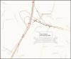
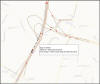
Problem 2: Operational analysis of the I-87/Alternate Route 7 Interchange This problem focuses on the interchange complex on the western end of Alternate Route 7. Three interchanges are intertwined: I-87 and Alternate Route 7, I-87 and State Route 2, and Alternate Route 7 and U.S. 9. Click the thumbnails of Exhibit 4-17 and Exhibit 4-18 for a visual introduction to this problem. Before proceeding with this problem, we first provide more details on the interchange geometry below. The interchange between I-87 and Alternate Route 7 is a classic trumpet with the semi-direct ramp linking Alternate Route 7 west to I-87 south. Locally, it’s called Exit 7, as noted in Exhibit 4-18. The one nuance worth noting is that the right-hand ramp from Alternate Route 7 west to I-87 north leaves Alternate Route 7 east of U.S. 9 and follows a fairly long path on its way to I-87 north. The Alternate Route 7/U.S. 9 interchange is a partial-cloverleaf. The connections to Alternate Route 7 east are on the eastern side of U.S. 9 while the connections to Alternate Route 7 west are on the western side. An extra ramp is needed to provide the connections, because the right-hand ramp from Alternate Route 7 to I-87 starts east of the bridge under U.S. 9, before the ramps from U.S. 9 connect to Alternate Route 7. Consequently, to provide connection from U.S. 9 via Alternate Route 7 to I-87, an extra ramp diverges from the U.S. 9 on-ramp north of NYS-7 and connects directly to the right-hand ramp from Alternate Route 7 west to I-87 north. The interchange between I-87 and State Route 2, Exit 6, is a simple diamond. It’s called Exit 6 as labeled in the diagram. Getting to it coming southbound is a bit complex. That needs a short discussion. |


Page Break
|
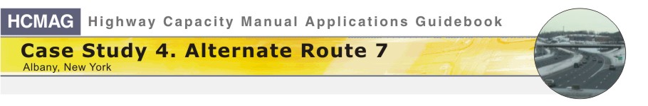
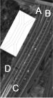
I-87/Alternate Route 7 Interchange (Note: Move the cursor over this aerial photograph to find hotspots that will allow you to see more detail of the interchange with a ground level photograph. The hotspots are highlighted by a dashed line rectangle in the figure below.) Starting at the top of the image and working south, we see the following things. First there are the exit ramps to Exits 6 and 7. The sliver of white is the gore that separates the two exit ramp lanes from the three main lanes. Next is the loop ramp to NYS-7 east. Then you can see the short single-lane connector that takes traffic going south to Exit 6 go from the diverge with the loop ramp to the merger with the semi-direct ramp. Starting at the southern end of the picture and working north, you can see Sparrowbush Road that crosses over the weaving section just north of Exit 6. Then you can see the point where the right-hand ramp diverges to NYS-7 east. To the right you can then see the interchange between NYS-7 and U.S. 9. On the south side of NYS-7 are the ramps to and from the eastbound direction. On the north side are the ramps to and from westbound direction. Also visible is the ramp short connector we described earlier that allows a connection from U.S. 9 to I-87 northbound. Click here to see an aerial photograph with key locations noted. |
 |
Page Break
|
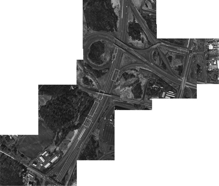
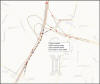
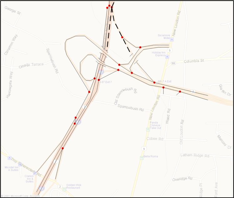
Exhibit 4-18. Interchange sketch. The six dashed-line rectangles in the figure below are hotspots. Click in these boxes to see a more detailed ground level photograph of that area of the interchange. |
 |
Page Break
Problem 2: Operational analysis of the I-87/Alternate Route 7 Interchange Looking again at Exhibit 4-18, you can see that all southbound vehicles wanting either Exit 6 or Exit 7 have to leave I-87 at the top of the diagram. Those going to Alternate Route 7 east diverge where the loop ramp turns west. Those going to Exit 6 continue south. Vehicles coming south from I-87 toward Exit 6 weave through the vehicles from the semi-direct ramp to I-87 south. A high percentage of vehicles on the semi-direct ramp have to cross the I-87 traffic going to Exit 6 then use the single lane slip ramp south of Location C to get to I-87. This difficult weave is one of the places analyzed in this problem. Now that you know some important details on the geometry of the interchange, let's consider the problem at hand, the completion of an operational analysis of the interchange. We will consider two specific procedures from the HCM, one to analyze weaving sections and the other to analyze ramp junctions. We will illustrate these two procedures using the four sub-problems listed below.
Sub-problem 2a. What
types of analysis should be conducted on the I-87/Alternate Route 7 interchange? |
Page Break
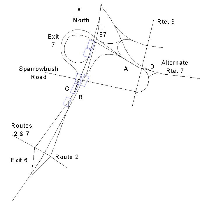
Sub-problem 2a: What types of analysis should be conducted on the I-87/Alternate Route 7 interchange? Step 1. Setup We first need to determine the types of analysis that we will conduct on the I-87/Alternate Route 7 interchange. We know from the HCM 2000 that there are four facility types: a basic freeway segment, a ramp junction, a weaving section, and a freeway facility (in which the three previous types are integrated together into a facility). One of the common challenges in a traffic analysis is to match the geometry found in a real problem with the four facility types described in the HCM. It is useful as we start this problem to determine which types of facilities are present in this interchange as we have defined it. Exhibit 4-19 shows the interchange, both with a base map showing the named roadway segments and a schematic showing how the road segments intersect. Each of the schematic links is on the mainline of the freeway, a connector roadway, or a ramp. Study the map to better familiarize yourself with the components of the interchange.
Discussion: |
Page Break
|
I-87/Alternate Route 7 Interchange.
|
Page Break
Sub-problem 2a: What types of analysis should be conducted on the I-87/Alternate Route 7 interchange? Step 2. Results The I-87/Alternate Route 7 interchange is complex. To evaluate the operations of this interchange, we need to break it down into several components, either weaving sections or ramp junctions. A weaving section is a segment of an uninterrupted flow facility (often a freeway) that requires a high proportion of vehicles to change lanes to reach their desired locations on the freeway. A weaving section is further characterized by the number of lanes in the weaving section, the length of the section, the number of lane changes required of the weaving traffic, and the type of terrain or grade. A ramp junction is the intersection of an on-ramp or off-ramp with a freeway, a point at which traffic either merges onto the freeway or diverges from the freeway. Similar to a weaving section, there is a higher degree of turbulence in the traffic stream near a ramp than in sections of the freeway that are longer distances away from a ramp or interchange. While an on-ramp at the beginning of a weaving section or an off-ramp at the end of a weaving section can also be analyzed as a ramp junction, the traffic stream characteristics present in a weaving section are more complex than would be present at a ramp junction alone. Thus, a separate procedure is needed to properly evaluate the effects of this higher degree of turbulence in the traffic stream. |
Page Break
Sub-problem 2a: What types of analysis should be conducted on the I-87/Alternate Route 7 interchange? Let's first list the ramp junctions present in the interchange. From Exhibit 4-19, we can see there are a total of sixteen ramps in our current study area:
However, only three of the locations represent true freeway merge or diverge points:
|
Page Break
Sub-problem 2a: What types of analysis should be conducted on the I-87/Alternate Route 7 interchange? These points can be analyzed using HCM Chapter 25. The other points can also be evaluated to determine the adequacy of their capacity, but the HCM procedures do not apply to the merge operations at these points. Note that the other merge and diverge points on the freeway segments that constitute this interchange are part of weaving sections and are discussed below. Let's now consider the weaving sections. They are composed of these on- and off-ramps that are no longer than 2,500 feet apart, or slightly less than one-half mile. If the ramps are spaced more than 2,500 feet apart, the turbulence resulting from the lane changing is limited to the vicinity of the ramps themselves, rather than being the combined effect of the on and off-ramps. There are three weaving sections in this interchange:
In order to assess the overall operation of the interchange, with its four ramp junctions and three weaving sections, we would need to evaluate the level of service at each one. However, in the interest of time, we will limit our focus here to the three weaving sections and one ramp junction. When you are ready, proceed to Sub-problem 2b. |
Page Break
Sub-problem 2b: What are the Levels of Service in the Weaving Sections Located in the I-87/Alternate Route 7 Interchange? Step 1. Setup In this sub-problem, we will consider the three weaving sections that are part of the I-87/Alternate Route 7 interchange and determine the quality of service that is provided to drivers traveling through these sections. These weaving sections, shown in Exhibits 4-20, 4-21, and 4-22, are classified as Type A weaves. As we begin this sub-problem, consider these questions:
Discussion: |
Page Break
|
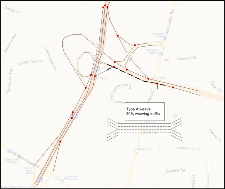
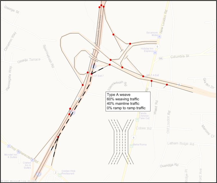
Exhibit 4-20. Weave A The beginning point of Weave A is defined by two entrance ramps to Alternate Route 7 eastbound, one from the circular loop ramp from I-87 southbound and one from the direct ramp from I-87 northbound. The end point of the weave section is defined by the point where the exit ramp to U.S. Route 9 leaves the EB Alternate Route 7 mainline. Weave A is a Type A weave. Why? In a Type A weave, both of the weaving traffic streams must change lanes once in order to reach their desired destination. Let's consider how this applies to Weave A. Traffic on the circular loop ramp from I-87 southbound desiring to travel to U.S. Route 9 must cross the crown line to reach this exit, and thus change lanes once. Similarly, traffic from the northbound I-87 exit ramp desiring to stay on Alternate Route 7 must change lanes once in order to be in the two left most lanes, the mainline for Alternate Route 7. The crossing of these two streams produces the turbulence that defines a weaving section. Local traffic engineers have estimated that 30 percent of the traffic entering the section is weaving, while 70 percent is through traffic or is not weaving.
|
Page Break
|
Exhibit 4-21. Weave B Weave B is located on I-87 northbound between the on-ramp from State Routes 2 and 7 on the lower left of the figure below (known locally as entrance 6) and the exit to Alternate Route 7 (known as exit 7). Weave B is a Type A weave. Why? Here, both weaving streams must change lanes once in order to reach their final destination. Traffic entering from State Routes 2 and 7 (entrance 6) must change lanes once in order to stay on the mainline I-87 northbound. Traffic on I-87 northbound desiring to travel to Alternate Route 7 eastbound must change lanes once to reach this off-ramp. Studies by local traffic engineers indicate that virtually no traffic entering from State Routes 2 and 7 also exit to Alternate Route 7 eastbound. They also estimate that 60 percent of the I-87 northbound traffic desires to exit to Alternate Route 7 eastbound, with the remaining 40 percent continuing on I-87 north past exit 7.
|
Page Break
|
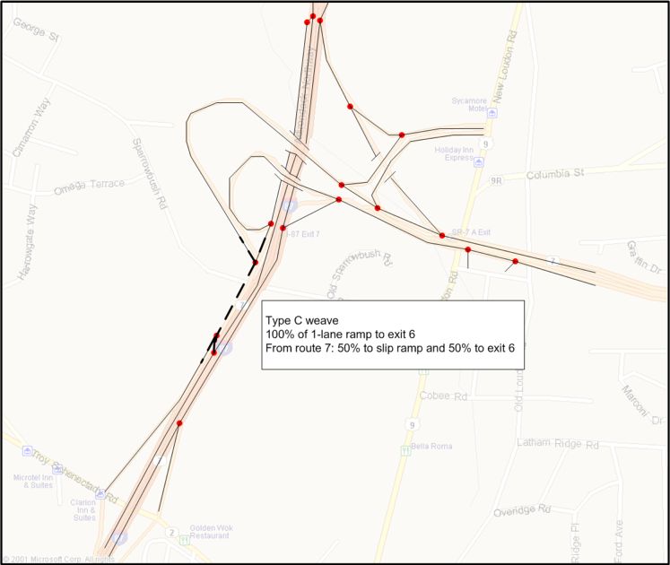
Exhibit 4-22. Weave C Weave C is formed by the I-87 southbound frontage road and the semi-direct ramp from westbound Alternate Route 7. The I-87 southbound frontage road and the slip ramp back to the I-87 mainline form the southern boundary of the weaving section. Weave C is a Type A weave. Why? In a Type A weave, both of the weaving traffic streams must change lanes once in order to reach their desired destination. Let's consider how this applies to Weave A. Traffic on the circular loop ramp from I-87 southbound desiring to travel to U.S. Route 9 must cross the crown line to reach this exit, and thus change lanes once. Similarly, traffic from the northbound I-87 exit ramp desiring to stay on Alternate Route 7 must change lanes once in order to be in the two left most lanes, the mainline for Alternate Route 7. The crossing of these two streams produces the turbulence that defines a weaving section. Local traffic engineers have estimated that 30 percent of the traffic entering the section is weaving, while 70 percent is through traffic or is not weaving.
|
Page Break
Sub-problem 2b: What are the Levels of Service in the Weaving Sections Located in the I-87/Alternate Route 7 Interchange? Now let's review each of these questions and discuss why they are relevant to this analysis. What type of analysis will produce an evaluation of traffic conditions present at the weaving sections? The Highway Capacity Manual (HCM) includes two kinds of analysis, depending on the problem that the analyst is attempting to address. An operational analysis produces an estimate of level of service, based on a detailed analysis of existing or projected traffic, geometric, and control conditions. A design analysis produces a value of a geometric parameter that will produce a given level of service. Here we will focus on an operational analysis of the weaving section. What data are needed to analyze the operations of these weaving sections? The weaving analysis procedure, documented in Chapter 24 of the HCM, requires the following input data:
|
Page Break
Sub-problem 2b: What are the Levels of Service in the Weaving Sections Located in the I-87/Alternate Route 7 Interchange? What are the limitations of the models used to analyze the performance of a weaving section? The weaving analysis procedure consists of five models or algorithms. Each of the models was developed and calibrated from several data sets collected from actual freeway operations. It is important when applying these sub-models to make sure the data that you are using fall within the following limits, which also define the limitations of the data sets upon which the models are based:
If your data are outside of these limits, it may imply that poor operations will result and that local queuing should be expected. Why are these weaving sections considered to be Type A weaves? The weaving section type is based on the number of lane changes that each of the weaving traffic streams must make in order to reach their final destination. In both of the cases here, each weaving traffic stream must make one lane change to reach its desired destination. For more discussion of the nature of the weaving traffic in the segments we are evaluating, refer to Exhibit 4-20 (Weave A), Exhibit 4-21, (Weave B), and Exhibit 4-22 (Weave C). What measures of effectiveness are used to evaluate the performance of a weaving section? Typically, the weaving analysis procedure is used to determine the level of service of the section, the number of lanes required to meet a specified level of service, the required length of the weaving section to meet a given level of service, or the type of weaving section configuration required to meet a given level of service. An operational analysis will produce the level of service, while a design analysis can be used to produce the other three outputs. For a weaving section, the level of service is defined by the traffic density. What is meant by the terms "constrained operation" and "unconstrained operation?" The determination of whether a particular weaving segment is operating in an unconstrained or constrained state is based on the comparison of two variables: the number of lanes that must be used by weaving vehicles to achieve equilibrium or unconstrained operation (Nw) and the maximum number of lanes that can be used by weaving vehicles for a given configuration (Nwmax). |
Page Break
Sub-problem 2b: What are the Levels of Service in the Weaving Sections Located in the I-87/Alternate Route 7 Interchange? The New York State Department of Transportation has a program of continuous traffic counting for most freeways and highways in the state. Data gathered from the permanent count stations located on the interchange were used to identify the morning and afternoon peak hour for the entry and exit points at the weaving sections, identified as points A, B, C, and D in Exhibits 4-24, 4-25, and 4-26 below. From these entry and exit counts, local traffic engineers estimated the origins and destinations for the weaving sections based on their knowledge of local traffic flow conditions. Sometimes you will have actual origin-destination movements for a weaving section, but other times, as for this sub-problem, you will need to estimate the weaving flows based on your knowledge of local conditions. Exhibit 4-23 shows the origin and destination data that were estimated for the three weaving sections.
|
|||||||||||||||||||||||||||||||||||||||||||||

Page Break
|
Exhibit 4-24. Weave A
|

Page Break
|
Exhibit 4-25. Weave B
|

Page Break
|
Exhibit 4-26. Weave C
|
Page Break
Sub-problem 2b: What are the Levels of Service in the Weaving Sections Located in the I-87/Alternate Route 7 Interchange? In addition to the volume data, we must also consider several other input data. For Weave A, the peak hour factor is used to account for the variation in the traffic flow during the peak hour. Based on previous studies, we will use a peak hour factor of 0.90. The free flow speed was estimated to be 55 (see previous discussion) mph while the proportion heavy vehicles is assumed to be zero for this analysis. We are also assuming the driver population adjustment factor to be 1.0. What about the geometric data? We've already determined that this is a Type A weave, according to the guidelines of the HCM. We also know from an examination of the aerial photographs and the schematics we reviewed earlier that there are four lanes in the weaving segment, two from each of the entry sections, and two going to each of the two exit sections. The length of the weaving section is 1,320 feet, or one-quarter mile. Weaves B and C are also Type A weaves. The input data for these weaving sections, as well as for Weave A, are summarized in Exhibit 4-27.
Discussion: |
||||||||||||||||||||||||||||||||||||||
Page Break
Sub-problem 2b: What are the Levels of Service in the Weaving Sections Located in the I-87/Alternate Route 7 Interchange? Step 2. Results The weaving analysis methodology of the HCM produces five distinct results:
The results of the weaving analysis are provided in Exhibit 4-28. After you've taken the time to review the data in Exhibit 4-28, consider the following questions:
Discussion: |
Page Break
|
||||||||||||||||||||||||||||||||||||||||||||||||||||||||||||||||||||||||||||||||||||||||||||||||||||||||||||||||||||||||||||||||||||||
Page Break
Sub-problem 2b: What are the Levels of Service in the Weaving Sections Located in the I-87/Alternate Route 7 Interchange? Let's now consider each of the questions posed on the previous page, referring again to Exhibit 4-28. How does the length of each weaving section affect its operation? Let's compare the results for Weaves A and B. In general, providing additional length in a weaving section allows drivers more time to complete their maneuvers (the intensity of lane changing decreases), often resulting in higher speeds in the weaving section. Thus, all other factors being equal, the degree of turbulence in Weave B should be lower than Weave A. However, since the volumes in Weave B are much higher than in Weave A, the overall weaving intensity is higher in Weave B, even with its greater length. The volume ratio, VR, is more than twice as high in Weaves B and C as in Weave A; is this significant and if so, why? The volume ratio is the ratio of the weaving flow rate to the total flow rate in the weaving section. As the proportion of weaving traffic increases, the degree of turbulence also increases. Two key results follow from this increased turbulence: speeds decrease and density increases. The volume ratio for Weaves B and C (ranging from 0.68 to 0.76) shows than between two-thirds and three-quarters of the total traffic is required to change lanes. This higher degree of turbulence in the traffic stream lowers vehicle speeds in the section, and you can see this result directly in the table shown on the previous page. What is the significance of the predicted speeds for the weaving and non-weaving traffic? The weaving speeds are approximately 16 to 18 mi/hr less than the non-weaving speeds for five of the time periods presented in the table; is this important and if so, why? Safer traffic flow always results if all vehicles in the traffic stream are traveling at the same speeds. While speed differentials are expected in a weaving section, the differences that we observe here are quite high, between 16 and 18 mi/hr. One of the factors that mitigates this speed differential in weaving sections is the degree of separation of the weaving traffic from the non-weaving traffic. Because of the nature of a Type A weave, all of the lane changing activity occurs in the two lanes adjacent to the crown line, with little or no spillover effects in the outer lanes. |
Page Break
Sub-problem 2b: What are the Levels of Service in the Weaving Sections Located in the I-87/Alternate Route 7 Interchange? Why is the weaving traffic constrained? What is the practical implication of this finding? (see Exhibit 4-28). The determination of whether a particular weaving segment is operating in an unconstrained or constrained state is based on the comparison of two variables: the number of lanes that must be used by weaving vehicles to achieve equilibrium or unconstrained operation (Nw) and the maximum number of lanes that can be used by weaving vehicles for a given configuration (Nwmax). As we have discussed previously, most, if not all, of the lane changing activity associated with weaving occurs in the two lanes adjacent to the crown line. In fact, for a Type A weave, the number of lanes that can be used by weaving vehicles is 1.4. It is less than 2 since some of the non-weaving vehicles also use these two lanes. Our results show that Weave A requires 1.5 lanes (fairly close to the number required for unconstrained flow), while Weave B requires from 3.3 to 3.6 lanes. Clearly, the volumes and proportion of weaving flow associated with Weave B requires much more space than is present in this type of weave, so the weaving traffic is definitely constrained. What happens when the weaving flow rate exceeds the model limit? When weaving flow rates exceed the model limits (in this case, 2,800 pc/hr for a Type A weave), it is likely that the weaving section will fail, regardless of the results from the other parts of the weaving section methodologies. For Weave B, during the PM Peak, the weaving volume is 4,105 pc/hr, a rate significantly higher than than 2,800 limit cited above. Again, the practical result is a likely breakdown of flow in this segment during this time period. In Weaves B and C, the volume ratio, VR, exceeds the model limit; what is the likely result that you would observe in the field? For weaving sections with five lanes, as in Weave A in this sub-problem, the volume ratio limit is 0.35. Both the AM and PM peak results are less than 0.35 for Weave A. However, for Weave B, the limit of 0.20 is exceeded in both the AM and PM peak periods. In fact, the values of 0.70 and 0.68 are significantly higher than the limit with a likely result of poor operations and local areas of queuing. The questions that we discussed above are important in helping us to understand how the three weaving sections will operate under the given conditions. As you consider all of the data together, how would you summarize the operations of the three weaving sections? After you have considered this question, proceed to the next page for a further discussion of this issue. |
Page Break
Sub-problem 2b: What are the Levels of Service in the Weaving Sections Located in the I-87/Alternate Route 7 Interchange? After a review of Exhibit 4-28 and the discussion from the previous page, we can summarize the operations of the three weaving sections as follows. Weave A is forecasted to operate at levels of service A and B during the AM and PM peak periods, respectively. While there is a high speed differential between the weaving and non-weaving vehicles, the proportion of weaving traffic (volume ratio) is low (0.31 and 0.30, respectively) during the two time periods. This means that the overall speed of all vehicles in the section is over 50 mi/hr and the resultant densities (9.4 pc/mi/lane and 12.5 pc/mi/lane) are low. We can conclude that, based on today's volumes, Weave A will operate at a very acceptable level for motorists traveling through this section. There is no reason to consider any changes to the design of this weaving section. We should further note that all model limitations are met by the conditions for Weave A, so we can be reasonably confidant of our conclusions. Weave B, by contrast, is forecasted to operate at level of service B during the AM peak but only level of service E during the PM peak period. What are the factors that cause this poor operation during the afternoon period? |
Page Break
Sub-problem 2b: What are the Levels of Service in the Weaving Sections Located in the I-87/Alternate Route 7 Interchange? By referring once again to the summary of results presented in Exhibit 4-28 we see much higher flow rates in the PM peak than in the AM peak, 5,447 veh/hr in the PM and only 2,196 veh/hr in the AM. And, while there is a very high volume ratio (VR) during both periods, the lower total volumes mitigate this condition in the AM peak. However, in the PM peak, the high volume ratio combined with the high overall flow rates result in an overall speed of 31.7 mi/hr in the weaving section and a density of 38.2 pc/mi/lane. Furthermore, both the volume ratio and the total weaving volume model limits are exceeded during the PM peak. The likely result is a breakdown of operations and queuing at some locations in the section. We should note that the volume ratio limit is also exceeded in the AM peak, again resulting in poor operations. We can conclude that, even though the forecasted level of service is B for the AM peak, both time periods will experience poor operations with breakdowns in flow to be expected. While we won't consider this sub-problem in more detail here, it would be valuable for you to review the results presented here and identify geometric improvements that you think might improve the operational performance of this weaving section. The operation of Weave C is even worse, with forecasts of level of service F for the AM peak and level of service E for the PM peak. With the high density and the failing conditions present for this analysis, we might ask whether or not we should consider another tool in addition to the HCM, such as a microscopic simulation model, to evaluate this weaving section. We will discuss this issue in more detail in Problem 5 of Case Study 4. |
Page Break
Sub-problem 2c: What is the Level of Service at the Ramp Junction at the Northbound On-Ramp to I-87? Step 1. Setup In this problem, we will consider the merge point between I-87 northbound and the ramp from westbound Alternate Route 7. The ramp itself is complex since it also has a merge point with the intersection of the on-ramp from U.S. 9. You can learn more about the ramp by clicking on the Exhibit caption. As we begin this sub-problem, let's consider several issues that relate to the analysis of a freeway ramp junction:
Discussion: |
Page Break
|
Merge point This merge point is formed by the intersection I-87 northbound mainline and the ramp from Alternate Route 7 westbound.
|
Page Break
Sub-problem 2c: What is the Level of Service at the Ramp Junction at the Northbound On-Ramp to I-87? Let's now consider each of these questions: Should we consider only the vicinity of the junction itself, or are there other areas that we should consider as well? The ramp junction methodology focuses on what is called the merge influence area. The merge influence area is defined as the area from the merge point to 1,500 feet downstream for lanes 1 and 2 of the freeway mainline. It is within this area that most of the effect of the merging traffic into the freeway mainline is observed. For this problem, this area is on I-87 from the point of the ramp merge to 1,500 feet downstream. But we should also consider other parts of the ramp itself. For example, the merge with the U.S. 9 ramp creates some turbulence in the traffic stream as the two ramps come together and drop from two lanes to one in a very short distance. Additionally, we must consider the capacity of the ramps themselves. We'll discuss each of these points later in the sub-problem. One other point must be made. When we are considering a merge analysis, we need to look at the location of adjacent on-ramps and off-ramps. If these ramps are within 1,500 feet, the effect that they have on the lane distribution of traffic must also be considered. Since there are no ramps within 1,500 feet of this merge area, this issue is not relevant to this problem. |
Page Break
Sub-problem 2c: What is the Level of Service at the Ramp Junction at the Northbound On-Ramp to I-87? What input data is needed to conduct this analysis? To conduct an operational analysis of a merge area, we need to have the following input data:
What the primary measure of effectiveness for a merge point analysis? We are conducting an operational analysis, so we want to be able to forecast the level of service of the merge influence area. The HCM uses density as the primary measure of effectiveness from which to determine the level of service. Density is expressed in terms of vehicles per mile per lane. What parameters are forecasted by the merge point analysis models in the HCM? To forecast the density of traffic in the merge influence area, the HCM uses several steps (and models). First, the flow rate in the merge influence area is computed. Recall that this is the flow rate in lanes 1 and 2 in the area just downstream of the merge. Next, the density in the merge area is computed and the level of service is determined. Finally, the speed is computed. What are some of the limitations of the merge point analysis model that we must keep in mind when applying it to this sub-problem? One of the major limitations of the ramp junction procedure in the HCM is that it does not apply when demand exceeds capacity. If demand exceeds capacity, we need to consider another procedure, possibly microscopic simulation. |
Page Break
Sub-problem 2c: What is the level of service at the ramp junction at the northbound on-ramp to I-87? Step 2. Results The input data for this problem is gathered from several sources. We can use the aerial photographs in Exhibit 4-17 and the map in Exhibit 4-18 that were presented earlier in this problem to determine the number of lanes on the I-87 mainline and on the ramp itself. The length of the acceleration lane was also determined from the map and aerial photos. We determined the free flow speeds on the freeway and on the ramp using data collected previously by the New York State DOT. The volume data is a topic that is worthy of additional discussion. While we could use ground counts collected by the DOT, we must be careful. Why? These counts represent service volumes, or the actual volumes using the facility during a given time interval. However, to have a true estimate of the facility performance, we must instead consider demand volume, or the number of users of a given segment during a specific period of time. Particularly when congestion exists, it is often difficult to estimate demand volume. Remember that the distinction between demand and volume is this: demand is the number of system users desiring service over the course of a given time interval, whereas volume is the number of system users actually served during that same time interval. With this distinction in mind, you can see that demand and volume are equivalent to one another only when the system is operating in an undersaturated mode. The data used for this problem are summarized in Exhibit 4-30.
Continue to the next page to see the results of applying the HCM ramp junction analysis to the conditions found in these two time periods. |
||||||||||||||||||||||||||||||||
Page Break
Sub-problem 2c: What is the level of service at the ramp junction at the northbound on-ramp to I-87? The data produced from the HCM analysis of the merge point located at northbound I-87 and the on-ramp from Alternate Route 7 westbound are shown in Exhibit 4-31.
Carefully study the information presented in the table. Using this information, consider the following questions:
Discussion: |
|||||||||||||||||||||||||||||||||||||||||||||||||||
Page Break
Sub-problem 2c: What is the level of service at the ramp junction at the northbound on-ramp to I-87? Let's now consider the questions from the previous page and Exhibit 4-31. What is the significance of the parameter, PFM? One of the most important functions of the merge point analysis is to estimate the lane distribution of traffic in the vicinity of the merge point. The proportion of the approaching freeway flow remaining in lanes 1 and 2 immediately upstream of the merge point is noted as PFM. This parameter depends on both the number of lanes on the freeway mainline and the length of the acceleration lane from the ramp to the mainline. For this particular analysis, the value of PFM is 0.59. This means that 59 percent of the approaching freeway flow remains in lanes 1 and 2 immediately upstream of the merge point. If the freeway had more lanes at this point, this value would be lower, as more of the mainline traffic would avoid the turbulence of the merge area. Which data from Exhibit 4-31 describe the nature of the flow of traffic in the merge influence area? Several model outputs help us to understand the nature of the flow in the merge area. The flow rate in the merge influence area (vR12) is compared to the capacity of the area to determine whether this area is under capacity or over capacity. The density and speed of the merge area is also computed; the density is used to determine level of service. |
Page Break
Sub-problem 2c: What is the level of service at the ramp junction at the northbound on-ramp to I-87? Note that the during the PM peak, vR12 is 5,265 passengers cars per hour, a flow rate which exceeds the capacity of the merge influence area (4,600 pc/h). The implication is important: a significant part of the demand (5,264 - 4,600 = 664) can't be served during the analysis period. This unserved demand is diverted to the next analysis period. The density during the PM peak is 42.4 pc/mi/lane, while the speed is forecasted to be just below 42 mi/hr. What is the basis for the forecast of level of service? The basis for forecasting level of service is the density of traffic flow. For this case, the density during the PM peak is 42.4 pc/mi/lane, which is level of service F. The level of service during the AM peak is B, based on a density estimate of 13.7 pc/mi/ln. How would you describe the operation of the merge point in the PM peak period? The operation of the merge point during the PM peak period is poor. The demand exceeds the capacity, the density is high, and the speed is relatively low. Since the demand exceeds capacity, we need to consider another analysis tool, such as a microscopic simulation tool, that will enable us to have a more accurate characterization of the operational performance of this ramp junction during the PM peak period. Remember that the HCM states in chapter 25 that this methodology does not take into account oversaturated conditions. The use of micro-simulation will be illustrated in problem 5 of this case study. |
Page Break
Sub-problem 2d: How Can We Improve the Level of Service at the Ramp Junction at the Northbound On-Ramp to I-87? Step 1. Setup The merge point that we considered in sub-problem 2c was over capacity during the PM peak hour. Queues extended over much of the length of the ramp. The demand exceeded capacity and the HCM methodology couldn't be used for this analysis under conditions present during the PM peak hour. But while the HCM methodology couldn't forecast the performance, we do know that the facility will fail since the demand was found to exceed capacity. Consider how we could mitigate this problem. What possible changes in the design of the ramp merge area should be considered? To provide insight into possible geometric mitigations, we can look more closely at the forecast models. There are five variables of prime importance:
Many factors determine whether or not changing any of these variables is feasible. But we can use the HCM procedure to determine how much change we can expect in the operational performance if one or more of these variables is modified. Discussion: |
Page Break
Sub-problem 2d: How Can We Improve the Level of Service at the Ramp Junction at the Northbound On-Ramp to I-87? We will explore three possible mitigation options in this sub-problem: adding a lane to the freeway mainline; adding a lane to the ramp; and lengthening the acceleration lane. Each of these mitigations requires minor changes in the input data. If we add a lane to the freeway mainline, one parameter change is required: the number of lanes on the freeway mainline. If we add a lane to the ramp, again, one parameter change is required: the number of lanes on the ramp. Similarly, if we change the length of the acceleration lane, this parameter must be modified. In the next several pages, we will consider the results of these parameter changes. You can follow the solutions and relevant discussion for each of these three changes through the links below: Adding a lane to the freeway mainline |
Page Break
Sub-problem 2d: How Can We Improve the Level of Service at the Ramp Junction at the Northbound On-Ramp to I-87? Step 2. Results Exhibits 4-32 and 4-33 show the impact of adding a lane to the freeway mainline. Exhibit 4-32 shows the input data while Exhibit 4-33 shows the output data produced from the HCM analysis.
After reviewing the output data shown in Exhibit 4-33, consider the following questions:
|
||||||||||||||||||||||||||||||||||||||||||||||||||||||||||||||||||||||||||
Page Break
Sub-problem 2d: How Can We Improve the Level of Service at the Ramp Junction at the Northbound On-Ramp to I-87? Exhibit 4-34 shows the results of adding a lane to the freeway mainline, with a direct comparison to the conditions before the lane was added. The most direct result of adding a lane is the increase in the mainline capacity from 6,750 to 9,000 pc/h. This has several related impacts. The proportion of approaching freeway flow remaining in lanes 1 and 2, PFM, decreases from 0.59 to 0.08, because the traffic remaining on the mainline is more likely to avoid the congestion inherent in the merge area: two lanes are now available for through traffic rather than one in the before case. This also shows in the traffic in the merge influence area (lanes 1 and 2 plus on-ramp), VR12, decreases from 5,265 to 2,526. After the lane is added, this flow rate is below the maximum (capacity) of 4,600. The overall performance of the merge area increases dramatically from LOS F before to LOS C after the addition of the lane. The speed of vehicles in the ramp influence area increases from 41.6 to 50.8 mph. This change has a clear and dramatic effect in the performance of the freeway.
|
|||||||||||||||||||||||||||||||||||||||||
Page Break
Sub-problem 2d: How Can We Improve the Level of Service at the Ramp Junction at the Northbound On-Ramp to I-87? Exhibits 4-35 and 4-36 show the effect of adding a lane to the ramp so that two lanes are maintained on the ramp for its entire length from Alternate Route 7 to I-87 North.
After reviewing the output data shown in Exhibit 4-36, consider the following questions:
Discussion: |
||||||||||||||||||||||||||||||||||||||||||||||||||||||||||||||||||||||||||||||||
Page Break
Sub-problem 2d: How Can We Improve the Level of Service at the Ramp Junction at the Northbound On-Ramp to I-87? A review of Exhibit 4-36 shows some minor improvements in the operational performance of the merge area. The density is reduced from 42.5 to 34.7 and the speed of the ramp influence area increases from 41.6 to 44.5 mph. But should we believe these forecasts? No. Since the forecasted volume in the merge area (5,070) exceeds the capacity (4,600) of the area, we know that the model cannot be applied realistically to these conditions. Thus, while we can produce output results, we need to know that in this case, the results cannot be used with any degree of certainty to help us with this analysis. Again, if we desired to have a more definitive assessment of the performance of this alternative, we would have to use another analysis tool, perhaps a microscopic simulation tool. Continue on to the next page to view the effect of extending the length of the acceleration lane on the performance of the merge area. |
Page Break
Sub-problem 2d: How Can We Improve the Level of Service at the Ramp Junction at the Northbound On-Ramp to I-87? Exhibit 4-37 shows the effect of increasing the acceleration lane from 500 (existing condition) to either 1,000 feet or 1,500 feet. Again, as with the addition of a lane to the ramp, the effect is not significant. In fact, as we saw before, the demand still exceeds the capacity of the merge influence area and so, here again, we cannot depend on the results from the HCM model for this analysis.
|
|||||||||||||||||||||||||||||||||||||||||||||||||||||||||
Page Break
Problem 2: Analysis We have produced a significant amount of information about the operation of the I-87/Alternate Route 7 interchange using the HCM. Let's summarize the key points from the four sub-problems we've just completed. In sub-problem 2a, we divided the interchange into manageable components that could be analyzed using the procedures of the HCM, including both weaving sections and ramp junctions. In sub-problems 2b, 2c, and 2d, we analyzed the operation of the three weaving sections and one of the four ramp junctions. Exhibit 4-38 summarizes the results of these analyses.
Weave A, the section of eastbound Alternate Route 7 from the I-87 on-ramp to the US 9 off-ramp, operates at an acceptable level of service A during the AM peak hour and B during the PM peak hour. In both cases, we can have confidence in the model forecasts, since the model's boundary conditions are satisfied. At both Weaves B and C, however, poor levels of service are forecasted, and the model conditions are not satisfied. We can assume that field conditions are poor with periodic queuing and delays for motorists traveling through these weaving sections. We also forecasted levels of service for the northbound I-87/Alternate Route 7 merge point. During the AM peak, the level of service is expected to be B, certainly an acceptable level of performance. However, for the PM peak hour, the level of service is forecasted to be F. Further, the demand exceeds the capacity, implying that the HCM model should not be applied for these conditions. |
|||||||||||||||||||||||||||||||||||||||||||||||||||||
Page Break
Problem 2: Discussion There are several issues that we should consider as part of the analysis we have just completed. First, while we have completed an analysis of the major components of the I-87/Alternate Route 7 interchange, we don't have results that we can say are completely reliable. For two of the weaving sections and for the ramp junction, the model boundaries were exceeded, thus putting some uncertainty on the results produced by the HCM analysis. Second, while we have looked at the components of the interchange, we are still conducting this analysis in some isolation. How does the operation of the interchange affect the mainline section of I-87, particularly in the vicinity of the various ramp junctions? How does the interchange affect the operation of Alternate Route 7? These questions and issues dictate the need to consider two additional problems in this case study. In Problem 4, we will use the Freeway Systems methodology from Chapter 22 of the HCM to consider Alternate Route 7 as a system, from the I-87 interchange to the I-787 interchange. This system perspective, looking at how the individual components operate together, is important for several reasons. One of these is that drivers consider this perspective every time they use (or judge) the facility. Drivers do not generally think about the performance characteristics of individual pieces of the freeway system, and then use this to judge the overall quality of their driving experience. Rather, their perception of the quality of service they have received develops over time, and they would typically describe the freeway they drove on as a single entity as opposed to a sequence of individual elements. In Problem 5, we will use a micro-simulation model to help us study the performance of the segments of Alternate Route 7 that could not be adequately analyzed by the HCM, particularly those segments in which demand exceeded capacity. |