Problem 1: Basic Freeway Sections

Printable Version

Basic freeway sections are among the most elementary of all highway facilities. They are single-directional links that tie one freeway juncture to the next. The freeway junctures can be weaving sections, ramp junctions, or merge or diverge points. Basic freeway sections are quickly identifiable because there is no distinctive pattern to the lane changing, and no evidence exists of distinctive subordinate traffic streams, as there would be at a weave, a ramp, or a merge or diverge.

In this case study, two basic freeway sections exist on Route 7 between I-87 and I-787, both eastbound and westbound as shown in Exhibit 4-3. The basic freeway sections are approximately three miles in length and each direction has characteristics that are unique.

The eastbound AADT is about 29,700 and the peak hour volumes range up to about 3,250 in the AM peak and 2,400 in the PM peak.

The westbound section has an AADT of about 30,000 vehicles and peak hour volumes of approximately 2,400 veh/hr in the AM peak and 3,500 in the PM Peak.

In this problem, we'll use both of these directions to provide illustrations of a basic freeway analyses. The eastbound direction is fairly basic and will allow us to get familiar with the input variables and the outputs, and to see how changes in some of those variables influence the results. The westbound direction has some distinct characteristics that will allow us to look at issues related to the number of lanes available, the designation of truck climbing lanes, and grades.

Here are some points to consider as you read through problem 1:

What time periods do you think should be selected for doing an analysis of a basic freeway section? What are the two or three most important characteristics of this subarea that will likely define the operational performance of these basic freeway sections? Do the defining characteristics differ by direction? How is the configuration of each basic freeway section likely to affect downstream system elements like merge points, diverge points, and weaving areas?

Discussion:
Take a few minutes to consider these questions. When you are ready to continue, click continue below to proceed.

Problem 1: Basic Freeway Sections

In this problem, you will consider the following issues as you work through the computations for three sub-problems:

Sub-problem 1a: Traffic Flow Patterns
Variation in volumes
Variations in the PHF
Speed-flow relationship
Flow-Occupancy
Sub-problem 1b: Basic Freeway Section Analysis (Eastbound Section)
Selection of Appropriate Data
Basic Freeway Analysis
Sub-problem 1c: Analysis of the Westbound Freeway Section
Number of Travel Lanes
Truck Climbing Lanes
Effect of Grades on Analyses

Sub-problem 1a: Traffic Flow Patterns

Step 1. Setup

It is important to carefully determine what volume, peak hour factor, and speed values should be used in a basic freeway analysis. Ideally, a combination of values that “typify” the conditions that exist during the peak hour would be used. However, it’s often hard to determine what data represent “typical” conditions. Often, not enough data is available to determine what a typical condition is. That’s not a problem here because plenty of information is available. In Sub-problem 1a we will look at the traffic data that was collected over a year-long period.

Discussion:
The data collection in this case study represents atypical conditions, where traffic data along the study roadway has been monitored for years. If this were not the case, how many volume studies would need to be completed to ensure typical roadway conditions were sampled with some degree of confidence? What other ways might be available to account for the variability between data samples and typical roadway conditions? Also, observe the variation in recorded traffic volumes during similar time periods and consider the impact of this variation on roadway performance.

Sub-problem 1a: Traffic Flow Patterns

Flow Patterns
Just east of the bridge for Miller Road is a monitoring point used by the Capital District’s Traffic Management Center, run by NYSDOT Region 1 and the New York State Police. There is a double-loop, 20-foot speed trap in each lane, eastbound and westbound. The inputs from these traps are monitored 24-hours a day, 7-days a week. Because the data is archived, we were able to obtain a copy of the 15-minute data collected at this location for 27 months, from 00:00 on April 25, 2000 to midnight on October 31, 2002.

For purposes of the case study, we studied these data for the 2001 calendar year (Data points for 8,611 of the 8,760 hours in 2001 are shown in Exhibit 4-5, as the traps were out of service during the few remaining hours where no data is available.) and discovered some important things about the flow conditions. The first thing we learned relates to the flows themselves. As can be seen in Exhibit 4-5, the flow rate for a given hour varies widely. There is a diurnal trend that can be identified. The diurnal pattern has its minimum at 2-3:00 AM. The AM peak lasts from about 5-9:00 AM, and it looks like the flow in the eastbound direction is heavier in the AM peak than it is in the PM peak by almost 20%. The largest recorded volume in the AM peak in 2001 was approximately 3,480 veh/hr, recorded on day 311 between 7-8:00 AM.

Sub-problem 1a: Traffic Flow Patterns

The westbound direction shows a similar daily trend as can be shown in Exhibit 4-6. There is the same diurnal pattern with a smaller AM peak and a larger PM peak. The PM peak appears to begin at about 3-4:00 PM and persist until 5-6:00 PM. (The largest recorded westbound hourly volume in 2001 was 3,830 veh/hr on the 324^th day of the year between 4-5:00 PM.)

Sub-problem 1a: Traffic Flow Patterns

Peak Hour Factor
There are always other questions about the performance of such facilities such as the relationship between hourly volumes and the peak hour factor, speed-flow relationships and flow-density relationships.

Exhibit 4-7 shows the relationship between the hourly volumes and the peak hour factors. The data for the entire year are again plotted. The westbound direction is shown, and the eastbound plot is nearly identical. The average value for the peak hour factor tends to increase as the volume increases. There’s more variation in its value at low flows than at high flows. It ranges as low as 0.25 (that means there was flow in only the peak 15-minute time period) and it spans up to 1.0 for almost all volumes.

Sub-problem 1a: Traffic Flow Patterns

Speed-Flow
Exhibit 4-8 shows one of the lane-specific speed-flow relationships. It happens to be for Lane 1 Eastbound in the AM peak time period, but it is similar to all the other peak hour plots (i.e., for the other eastbound lane in the AM peak and for the westbound lanes in the PM peak). The mean speed stays at or near its maximum value (55 mph) from free flow conditions to capacity. Moreover, at the high flow rates there are conditions where the speeds are substantially lower as congestion impedes performance.

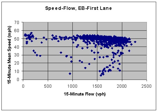
Sub-problem 1a:  Traffic Flow Patterns

Flow-Occupancy
Exhibit 4-9 shows the corresponding flow-occupancy relationship for the same lane and peak hour. The classical triangular shape depicted in textbooks is evident, with a positive, linear relationship from (0,0) up to a maximum of (15, 2264) between occupancy and flow for the uncongested conditions and then a downward sloping trend toward (100,0) for congested conditions during queue clearance.

All of these exhibits tell us we have a basic freeway section with typical variations in the flows and the flow conditions. Moreover, from Exhibits 4-5 and 4-6, it is apparent that the volume to select for the peak period analysis is not that obvious. The volumes during the peak hour tend to vary a great deal. In the AM peak hour (7-8:00 AM), for example, the volume ranges from about 200 veh/hr up to nearly 3,500 veh/hr. The average is about 2,000 veh/hr. None of these values seem to be correct for the analysis. The westbound volume during the PM peak hour (4-5:00 PM) range from about 750 veh/hr to 3,800 veh/hr, averaging about 2,000 veh/hr. Again, none of these values seem to be the best choice for a PM peak hour analysis. We can gain further insight into the issues associated with that choice by examining the flow rates associated with the four 15-minute time periods that occur during the AM and PM peak hours on weekdays during the year.

Sub-problem 1a: Traffic Flow Patterns

Trends in the Traffic Volumes
Exhibit 4-10 shows the distribution of weekday, 7-8:00 AM peak hour volumes for the eastbound direction. On the one hand, it is apparent that the volumes can be quite low. On the other, the values range up to 3,483 veh/hr. The mean value is 2,916 veh/hr and the 50^th-percentile is 3,096 veh/hr. The 90^th percentile is 3,340 veh/hr and the 95^th-percentile is 3,385. The question is, which value is the right one to select, one of these or some other?

Most traffic engineers would think about the mean value when they talk about a typical peak hour. But if you look at Exhibit 4-10, that seems like a pretty low value to use in assessing the facility’s performance. For illustrative purposes, in the next sub-problem we’re going to use the 90^th-percentile volumes instead of the average volumes. This means that the analysis results will represent conditions that will occur 90% of the year during the AM peak hour. (We’ll come back and look at the facility’s performance during the average peak hour conditions right after that.)

Sub-problem 1b: Analysis of the Eastbound Freeway Section

Step 1. Setup

In this sub-problem we will analyze a freeway section. The steps that we will use are outlined in Exhibit 4-11 below.

Discussion:
Take a few minutes to consider the figure above.  Click continue when you are ready to proceed.

Sub-problem 1b: Analysis of the Eastbound Freeway Section

The eastbound section has two lanes and is divided into three segments:

The first task is to specify the conditions. One important question is: where should we do the analysis? Should we use the 5-7% downgrade, the 1-2% upgrade, or the 1-2% downgrade? The HCM says: use the section that will produce the most conservative estimate of the LOS. That is, worst case governs.

So we’ll use the 1-2% upgrade section. In addition, because it is a mile long or more, we’ll assume it’s a constant grade, not a rolling or mountainous section. (As an aside, those categories don’t really have to do with where the facility is. They relate a lot more to the vertical profile of the segment. For example, a freeway running along a mountaintop is level even though it’s in a mountainous region.)

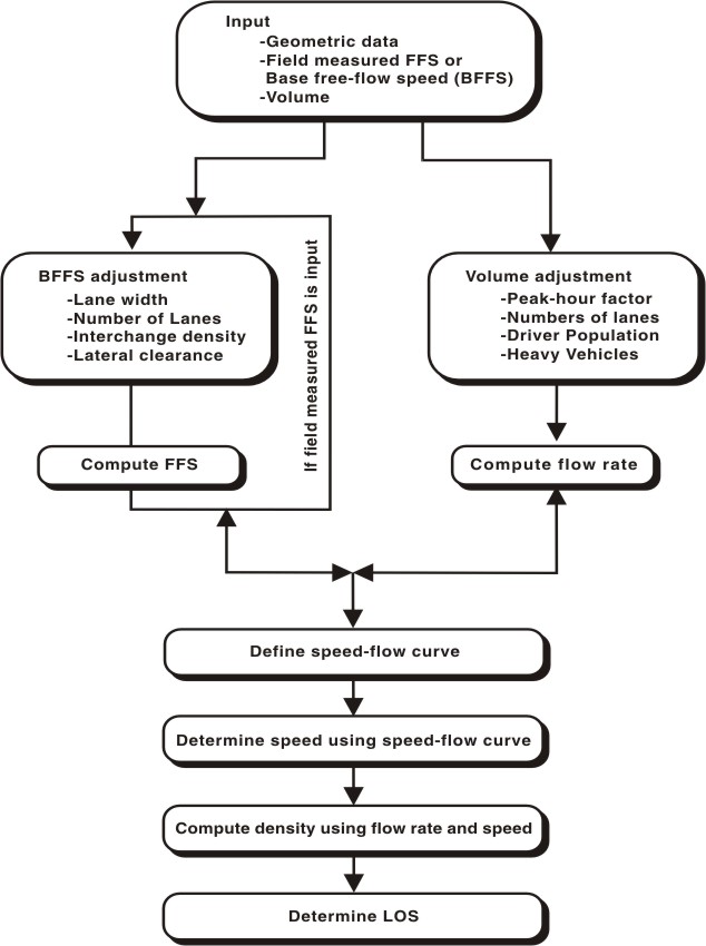
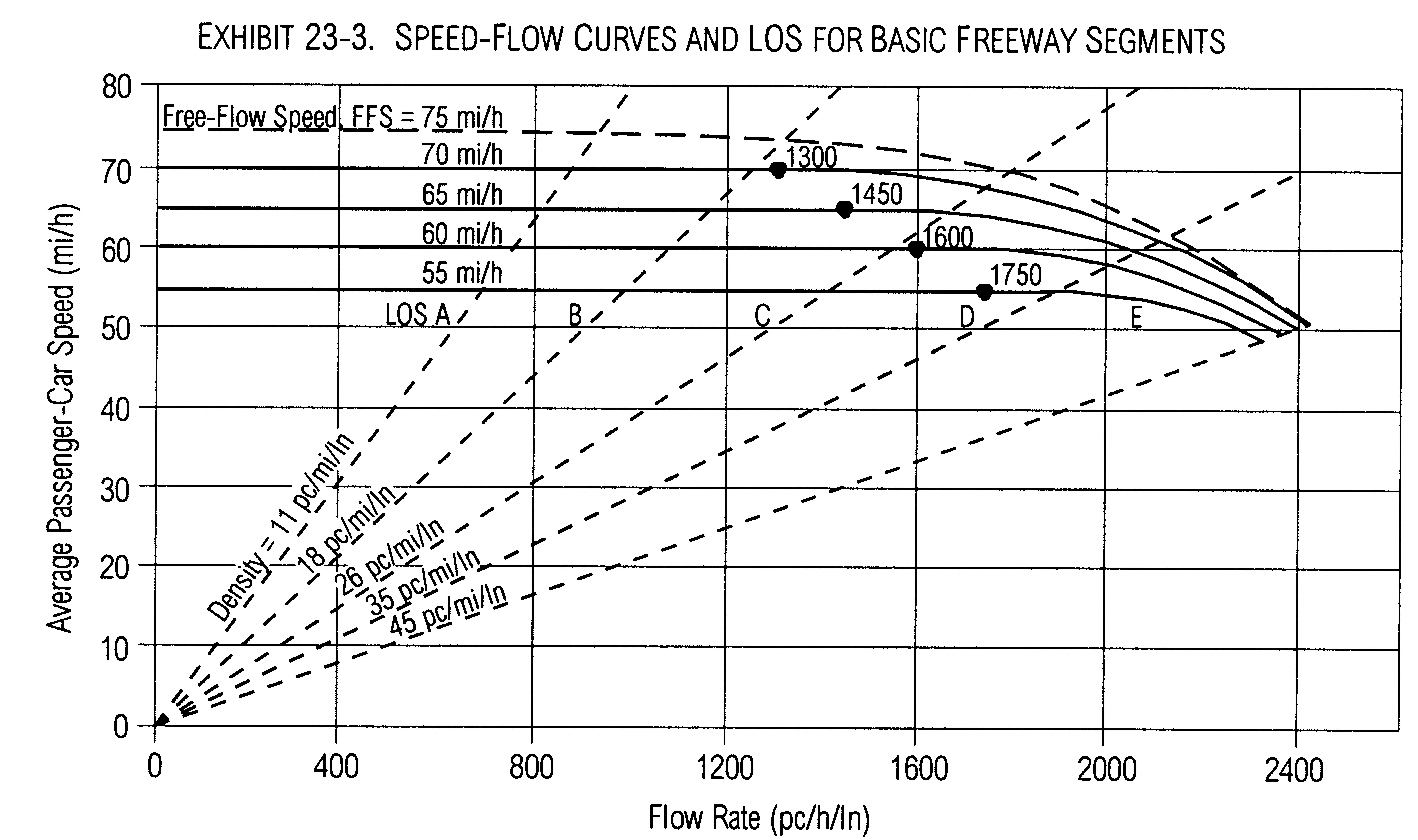
Sub-problem 1b: Analysis of the Eastbound Freeway Section

The basic freeway analysis methodology is shown in Exhibit 4-11. The inputs required include geometric data, a free-flow speed (FFS) (or a free flow speed derived from a basic free-flow speed) and volume information. The left-hand branch addresses actions you have to take to obtain the free-flow speed while the right hand branch focuses on the computation of a peak 15-minute flow rate. We’ll consider the left-hand branch first.

Free-flow speed (FFS) can be measured in the field or estimated using the procedure outlined in Chapter 23. We’ll consider both.

The benefit of having speed-flow data as shown in Exhibit 4-8 in this case study is that we can select a FFS and no adjustments are necessary. If you look at that figure, you can see that a value in the range of 55 mph is a good choice. This range reflects the average maximum speed when the flow rate relatively low. We’ll assume that 55 mph is the right value.

However, it’s useful to see what FFS estimate we would get if we trace through the branch labeled "if BFFS is input." We then take a basic free-flow speed (BFFS) and make adjustments to it to account for lane width, the number of lanes, the interchange density, and lateral clearances. Nominally, the basic free flow speed (BFFS) is how fast vehicles are traveling when the volumes are very light. The HCM assumes the BFFS is BFFS is 70 mph in urban settings and 75 mph in rural settings. Exhibit 4-8 shows that both of these values are too high for this facility. The maximum speed when the flow is almost zero is about 60 mph. The HCM allows us to use a local value rather than the defaults. We’re going to do that and assume the BFFS is 60 mph.

Sub-problem 1b: Analysis of the Eastbound Freeway Section

Using the method to calculate FFS based on BFFS as shown in Chapter 23, our FFS is projected to be 55.5 mph, which is very close to what the data shows us in Exhibit 4-8.

Now we need to revisit Exhibit 4-11 and see that the next thing to do is to calculate the peak 15-minute flow rate.

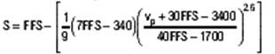
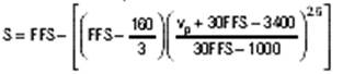
Sub-problem 1b: Analysis of the Eastbound Freeway Section

Since we don’t have any formal data for the percentage of trucks/buses or recreational vehicles in the traffic stream (during the peak hour), we’ll use anecdotal observations and say that the percentage of trucks/buses is about 5% (which means P_T is 0.05). We will assume there is no significant volume of recreational vehicles in the traffic stream.

Referring to Equation 23-2 in the HCM, we have V = 3,340 veh/hr, PHF = 0.90, N = 2, P_T = 0.05, P_R = 0, E_T = 1.5, E_R = 1.2, and f_p = 1.0. This gives us an average 15-minute passenger-car equivalent flow rate, v_p of 1,902 passenger cars per hour per lane.

There’s one more thing to do before we assess the level of service (LOS) for the facility, and that’s to compute the average passenger car speed as shown on HCM page 23-5, using a set of equations based on Exhibit 4-12.

The equations break the speed-flow relationship shown in Exhibit 4-12 into a set of regions delineated as follows:

Sub-problem 1b: Analysis of the Eastbound Freeway Section

The result for our situation is S = 54.8 mph. If you take this value and divide it into the peak 15-minute flow rate, v_p, then you get the freeway segment’s peak 15-minute average density (passenger cars per mile per lane), which is the basis for assessing the LOS (see Dataset 1):

          D = v_p / S = 1,902 pcphpl / 54.8 mph = 34.7 pcpmpl

Where pcphpl means passenger cars per hour per lane, mph is miles per hour, and pcpmpl is passenger cars per mile per lane. The breakpoints in D for level of service are as follows, all in passenger cars per mile per lane: A: 0-11; B: 11-18, C: 18-26, D: 26-35, and E: 35-45. Above 45 is LOS F.

For the circumstances we’ve examined, where D = 34.7, the LOS is a high D, almost E. Since we picked the 90^th percentile value to evaluate, this means that 10% of the time the eastbound LOS in the peak hour is D or worse, and 90% of the time it is better than that.

Three other significant conditions have the following levels of service:

If we want to more clearly characterize the performance of this location during the peak hour, we ought to evaluate its performance during all of the 256 peak hours (7-8:00 AM on a weekday) for which we have data. This isn’t a reasonable thought from a practical standpoint, but it gives us a way to make an important point.

Sub-problem 1b: Analysis of the Eastbound Freeway Section

The question we’re trying to answer is this: What is the performance of this facility like during a reasonably heavy AM peak hour (some might refer to this as the design hour)? To answer the question, we constructed a spreadsheet that implements the HCM methodology shown in Equations (1)-(4) in a single row of a spreadsheet. The spreadsheet contains a column for each of the following data items: day of the year, day of the week, hour, eastbound volume, eastbound PHF, percent trucks, percent recreational vehicles, heavy vehicle factor, driver population factor, peak 15-minute flow rate (v_p), passenger car speed, and density. Subordinate tables contain the lane width, the right-hand shoulder clearance, and the number of lanes.

Three of these data items are derived from the monitoring station data: V, the volume for the hour; PHF, the peak hour factor (since these can be computed from the underlying 15-minute data), and S the passenger car speed for the peak 15-minute time period. P_T is set to 5%, P_R is set to 0%, and f_p is set to 1.0

Our findings are shown in Exhibit 4-13 and Exhibit 4-14. For 208 of the 256 AM peak hours, or about 81.3%, the LOS is D. That’s significant news. The predominant LOS is clearly D. For 5.1% of the peak hours it is E, for 1.6% it is F and for 6.6% it is C. (The remaining 5.4% of the time it is A or B, probably on weekdays that are holidays.) This seems consistent with field observations.

The implications of Exhibit 4-13 are clear in terms of characterizing the performance of the facility. You can be comfortable describing its average condition as D. You could say that most of the time the LOS is D, in some heavily-traveled hours (6.7% of the time or about once every two weeks) the LOS is E or F, and the rest of the time it is A, B, or C. Chances are, your audience will understand that. Certainly, your fellow traffic engineers will.

Sub-problem 1c: Analysis of the Westbound Freeway Section

Step 1. Setup

We will now consider the conditions found along the westbound section, similar to sub-problem 1a. Before we begin, think about why conditions on the westbound section would be different than those on the eastbound section? Consider roadway users, physical conditions, and heavy vehicle needs.

Discussion:
Take a few minutes to consider the question above.

Sub-problem 1c: Westbound Peak Hour

The first task is to specify the conditions. The question again emerges: where should we do the analysis? Should we use the 6-7% upgrade, the 1-2% upgrade, or the 1-2% downgrade? The HCM says: use the section that will produce the most conservative estimate of the LOS. That is, worst case governs. So we’ll use the 6-7% upgrade section. In addition, since it is a mile long or more, we’ll assume it’s a constant grade, not a “rolling” or “mountainous” section.

For the other inputs, we’ll have the following values: 3 lanes, 3,240 veh/hr (the average PM peak hour volume), 55 mph as the free flow speed, 0.90 as the peak hour factor, 5% trucks/buses, and “local” drivers, i.e., ones that are familiar with the facility.

The results are as follows. A flow rate of 1,440 pcplph, a density of 26 pcplpm, a LOS of D, and an average passenger-car speed of 55 mph (see Dataset 5).

With this kind of output, we should see if two lanes would be enough. If we change the number of lanes to two, the flow rate becomes 2,160 pcplph, the density is 42 pcplpm, the LOS is E, and the average passenger car speed is 52 mph. The third lane has a huge impact on the results (see Dataset 6).

Let’s look at the issue about whether the truck-climbing lane is needed. While this specific issue is not addressed in the HCM methodology for basic freeway sections, we can analyze this by looking at the LOS for the section without the presence of the truck-climbing lane and comparing that to the LOS calculated if all trucks are removed from the passenger car travel lanes.

First, let's look at the truck-climbing lane. We effectively have 5% trucks, or 162 trucks per hour, in the peak hour volume. If the E_T is 5, as HCM Exhibit 23-9 suggests, the equivalent flow in passenger cars per hour is 810 passenger cars per hour. That illustrates the impact of the trucks. That’s almost a half lane’s worth of capacity.

Sub-problem 1c: Analysis of the Eastbound Freeway Section

You can compute the LOS by hand, but most software packages won’t let you do a single lane analysis directly. So you need to do a work-around. To begin, you can assume a volume of 1,620 passenger cars per hour and a two-lane facility. That yields a LOS of B and a density of 16.4 pcpmpl. So the truck climbing lane, if it’s used just by the trucks, operates adequately (see Dataset 7).

Next we need to check the remaining two lanes to see how they would operate if no trucks were present. The cars are 95% of the traffic stream, which means a volume of 3,080 veh/hour. On two lanes, with 0% trucks, that yields a per lane flow rate of 1,711 pcphpl, a density of 31.1 pcpmpl, and a LOS of D. The average passenger car speed is 55 mph (see Dataset 8).

Now let's consider the results of this hypothetical scenario. If we assume all three lanes are used by all the traffic, we get a density of 26.2 pcpmpl. If we separate the trucks into the truck climbing lane, we get 16.4 pcpmpl for the truck climbing lane and 31.1 pcpmpl for the remaining two auto-only lanes. These results suggest that trying to enforce exclusive use by trucks of the truck-climbing lane wouldn’t be a good idea.

Sub-problem 1c: Analysis of the Eastbound Freeway Section

Next, we should examine the impacts that result from varying other variables. If we increase the truck percentage to 10%, two things happen (see Dataset 9):

The fact that these two trends offset one another is a very important thing to notice.

To complete the sensitivity analyses, let’s look at the impacts from varying the driver familiarity adjustment factor. Let’s try using 0.85 instead of 1.0, assuming that the analysis is being done in the summer when a higher percentage of the drivers are vacationers. The flow rate becomes 1,695 pcphpl, the density becomes 30.8 pcpmpl, the LOS is D, and the average passenger car speed is 55 mph. This is a 17.6% increase over the value we found for the initial conditions we studied. So there is an impact on operations, even though the LOS is still D (see Dataset 10).

Sub-problem 1c: Analysis of the Eastbound Freeway Section

We can close out this analysis by looking at the performance of this facility across the entire year. As was the case for the eastbound analysis, we have data for 256 hours during 2001. The histogram, in Exhibit 4-15, shows that the predominant LOS is C, with some evidence of D, E, A, and B. It’s clear that you can describe the LOS of this westbound section as being predominantly C under the conditions we assumed: 5% trucks/buses, 0% recreational vehicles, and 0% daily users. If one or more of these assumptions change, the situation could be different.

To explore how different it might be, we changed just one variable, the assumption about daily users. We did this because during the spring, summer, and fall months many of the users on Friday afternoons are vacationers. If we change this assumption, the value of f_P can range as low as 0.85. The results of this analysis are presented below in Exhibit 4-16.

The percentage of hours at LOS F doesn’t change that much, from 2.0% to 2.3%, but the predominant LOS changes substantially, from C to D. Now 82% of the time, the LOS is D while only 7.8% of the time it is C.

Neither one of the situations, either “Regular Drivers” or “Vacation” drivers exactly describes peak hour situation. The truth is somewhere between. However, what we can say is that the LOS is typically either C or D. Moreover, it’s C-like during normal peak hours when the regular drivers predominate, and it’s D-like when the vacation drivers are present.