Problem 4: Analysis of the Alternate Route 7 Freeway Facility

Printable Version

In the previous three problems of this case study, we examined the operation of individual segments of Alternate Route 7, including basic freeway segments, weaving sections, and ramp junctions. In this problem, we will step back and consider the segments as drivers actually see them: part of a complete freeway facility. This perspective is also the way that the New York State DOT views this facility, a facility operating as a whole unit rather than separate components.

In addition, there are interactions between the various segments of this freeway that we have previously studied. For example, we earlier considered the weaving section that exists on eastbound Alternate Route 7 between the I-87 NB on-ramp and the U.S. Route 9 off-ramp on the western portion of the facility. A weaving section is by its nature a combination of two ramp junctions. Another example of the interaction between segments is when the flows from one part of the freeway interact with the flows from another part of the freeway. If a bottleneck exists, say as a result of a temporary lane closure, the flow from the bottleneck may spill back a mile or more upstream.

The question that we consider in this problem is how to determine the performance of the facility as a whole, then use this analysis to help us to identify (or verify) problems that exist in the field today.

We will consider three sub-problems to illustrate the application of the freeway facility analysis procedure.

Sub-problem 4a - How should the Alternate Route 7 facility be divided up for an HCM operational analysis?

Sub-problem 4b - What is the operational performance of Alternate Route 7 during the off peak period?

Sub-problem 4c - What is the operational performance of Alternate Route 7 during the peak period?

Continue with sub-problem 4a when you are ready.

Sub-problem 4a: Division of Alternate Route 7 for Analysis

Step 1. Set-up

The freeway facilities procedure (as documented in Chapter 22 of the HCM) uses component procedures (basic freeway segments, weaving sections, and ramp junctions) from three HCM chapters (23, 24, and 25) in an integrated manner to produce an assessment of the performance of the facility as a whole. The purpose of this sub-problem is to provide you with the experience of determining the appropriate segments for such an analysis. That is, how must we divide up the facility into manageable parts that will allow us to conduct an operational analysis using the methods of the HCM?

We need to divide the facility into both temporal and spatial segments. The time segments are usually the 15-minute time blocks typically used in an HCM analysis. The freeway is also divided into spatial segments whenever there is a change in the demand (because of an on-ramp or off-ramp) or capacity (number of lanes, grade change, etc). We further divide the segments into sections noting each of the standard HCM analysis procedures relevant to a section: basic section, ramp influence area, and weaving section. For example, consider a section of freeway, 5,000 feet in length, bounded by an on-ramp and an off-ramp. The section would be divided into a merge influence area 1,500 feet in length, a basic freeway segment 2,000 feet in length, and a diverge influence area 1,500 feet in length.

Sub-problem 4a: Division of Alternate Route 7 for Analysis

It is important that the time and space domain we establish includes time intervals during which any congestion or overcapacity may occur. For example, if the demand exceeds the capacity of a section for one 15-minute period, we need to continue the analysis for another time period in order for all of the demand to be served. In addition, we need to make sure that the overall length of the facility is such that vehicles are normally able to travel from one end to the other within 15 minutes, again so that all demand can be served during the study period. Finally, the facility should be long enough to contain any queues that form and to ensure that there are no traffic interactions with any upstream facility.

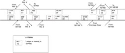
Now let's get started on this sub-problem and see how we can use these guidelines to analyze Alternate Route 7. Exhibit 4-63 shows line drawings of both the eastbound and westbound alignments of Alternate Route 7, from the I-87 interchange on the west to the I-787 interchange on the east. Study Exhibit 4-63 to better familiarize yourself with the components of this facility.
 

Discussion:
Consider the information presented in the line drawings above showing some of the geometric characteristics of Alternate Route 7. After reviewing the information included in the drawings, list the segments that you think should be analyzed. When you are ready, proceed to the next page.
 

Sub-problem 4a: Division of Alternate Route 7 for Analysis

Step 2. Results

Alternate Route 7 is a complex facility but if you follow the guidelines presented on the previous page, you should be able to identify the segments that make up the facility.

Let's start with the eastbound portion of the facility. We first look for factors that cause a change in either the demand or the capacity of the facility. The most common reason for a change in the demand is the presence of an on-ramp or off-ramp, where traffic either enters or leaves the facility. There are six ramps on eastbound Alternate Route 7. We should also note that between the I-87 and I-787 interchanges (specifically between the on-ramp from U.S. Route 9 and the off-ramp to I-787), there are two lane drops, each causing a reduction in the capacity of the facility. Thus, considering both the presence of ramps and the location of lane drops, there are nine sections along the eastbound portion of the facility.

Now let's consider the westbound portion of the facility. Again, there are six ramps, but since there are no lane drops or other factors that would cause a change in the capacity between the ramps, there are seven segments.

Remember that we also need to consider the three HCM analysis methods (basic freeway section, ramp influence, area, and weaving section) and determine how they apply. The eastbound portion of the facility includes a weaving section (remember our analysis in Problem 2 of this case study) and four ramp influences areas both in the merge area just downstream from the on-ramps and the diverge area just upstream from the on-ramps. The westbound portion includes six ramp influence areas, both merge and diverge areas. In total, there are eleven segments each for the eastbound and westbound portions of this facility.

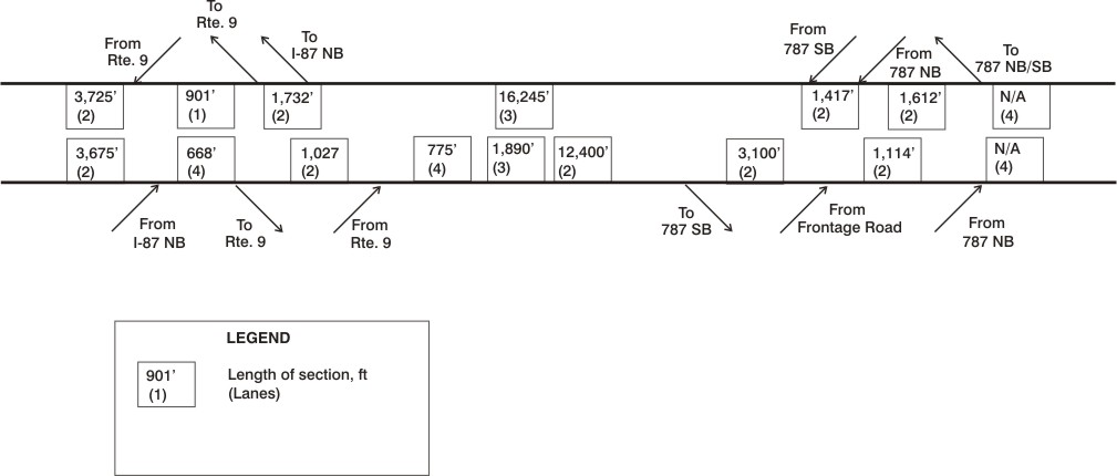
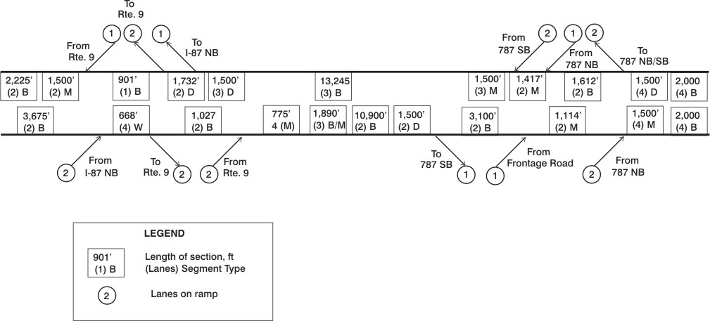
Sub-problem 4a: Division of Alternate Route 7 for Analysis

Check Exhibit 4-64 to see how well you did in identifying the segments that make up this facility. For each segment, Exhibit 4-64 includes the segment length, the number of lanes on the freeway mainline, and the segment type (either B for basic segment, M or D for merge or diverge area, or W for weaving section). It also includes the number of lanes on each of the on and off-ramps, shown in circles.

Study this information carefully. You should be able to see why each segment was defined. When you are ready, proceed to sub-problem 4b, where we will study the performance of this facility during the off-peak period.

Sub-problem 4b: Off-Peak Operational Analysis of Alternate Route 7

Step 1. Set-up

We'll now use the information that we developed in sub-problem 4a as the basis for an operational analysis of the facility. This information provides the spatial basis for our analysis, the division of the facility into segments. We'll focus our discussion primarily on the eastbound portion of the facility but will review the results of the analysis for the westbound portion as well.

Let's consider what constitutes an operational analysis of a freeway facility. When we conduct an operational analysis, we are interested in the performance of the facility at a fairly detailed level, with enough information so that the analyst can assess how the facility will function, given both the demand and geometric inputs. The HCM analysis for a freeway facility produces several performance measures, including speed and density, as well as an estimate of the capacity of each of the segments of the facility, based on these inputs.

In order to conduct this operational analysis, we will need the following input data:

Sub-problem 4b: Off-Peak Operational Analysis of Alternate Route 7

We've developed the geometric data previously, as part of sub-problem 4a. Let's now look at the traffic characteristics and demand data. From previous studies, the New York State DOT has assembled the following information on the traffic characteristics using this facility.

The demand data is extremely important for this analysis. And, again note that we use the term demand data or demand volume. While we typically measure service volumes in the field (the number of vehicles passing by our observation point during a specified time interval), we need to make sure that we have the actual number of vehicles desiring to use the facility, even if there is queuing present. Exhibit 4-66 includes the demand data for the eastbound portion of Alternate Route 7 for the midday period.

We also need the ramp-to-ramp weaving volume for the weaving section defined by the on-ramp from northbound I-87 to the off-ramp to U.S. Route 9. This demand is 1,625 veh/hr.

When you are ready to learn about the results of this analysis, proceed to the next page.

Sub-problem 4b: Off-Peak Operational Analysis of Alternate Route 7

Step 2. Results

The HCM freeway facility analysis produces a sizable amount of data. Exhibits 4-67 and 4-68 provides a summary of some of the key output data for the eastbound and the westbound sections respectively.

Sub-problem 4b: Off-Peak Operational Analysis of Alternate Route 7

Discussion:
Spend several minutes reviewing the data in Exhibits 4-67 and 4-68. What can you learn about the performance of the facility from these data? When you are ready, proceed to the next page.

Sub-problem 4b: Off-Peak Operational Analysis of Alternate Route 7

Step 2. Results

Let's first consider the level of service for the facility, or, more correctly, for each segment of the facility that makes up this analysis. We need to note that, using this method, there is no overall performance measure for the facility as a whole. Part 3 of the HCM does cover issues relating to corridor and area-wide analysis. But we will not cover them here. If you are interested in learning more about this topic, consult part 4 of the HCM.

The level of service for each segment is shown in Exhibit 4-69. Each of the segments performs at level of service C or better, with the exception of segment 2, the weaving segment. This result is consistent with our analysis produced in Problem 2 where we identified deficiencies with this weaving segment during the peak period. We also noted that, while speeds in other segments are nearly 50 mph or above, segment 2 has a forecasted speed below 28 mph, indicating a problem in the performance of the weaving segment.

We can also note that the demand/capacity ratio is near one for this segment. What is the implication of a demand/capacity ratio that is this high?

Sub-problem 4b: Off-Peak Operational Analysis of Alternate Route 7

When we examine Exhibit 4-70, which deals with ramp operations, we can see one of the results of the d/c ratio near one for the weaving segment (segment 02). Both the demands on the on- and off-ramps are not completely served during this time period. Note for example that the demand for the on-ramp is 2,835 vehicles, while the actual ramp volume is 2,100 vehicles. But there are two points to make here that limit the applicability of these results. First, a limitation in the software used to implement the HCM did not allow entry of 2 lanes to the on-ramp. This produces an unreasonable result of ramp delay and queuing. Second, if this limitation were not present and the results were as shown in Exhibit 4-70, the unserved demand during this time period would be transferred to the next 15-minute time period. The same caveat must be applied to the off-ramp results. So, while we can learn an important point about oversaturated conditions (demand exceeds capacity), this example does have a limitation (due to current software characteristics) that we need to keep in mind.

These results apply to the off-peak period. In sub-problem 4c, we will consider the peak hour operation of the facility.

Sub-problem 4c: Peak Operational Analysis of Alternate Route 7

Step 1. Setup

The operation of the facility during the peak period illustrates a very important point. What happens on the freeway mainline when the demand during one time period exceeds the capacity of the freeway to handle the demand. We will again consider only the eastbound portion of Alternate Route 7. The demand for four consecutive 15-minute time periods during the afternoon peak period is shown in Exhibit 4-71.

When you are ready to learn about the results of this analysis, proceed to the next page.

Sub-problem 4c: Peak Operational Analysis of Alternate Route 7

Step 2. Results

Exhibit 4-72 shows the results for the time period 1. Study these results carefully.

Discussion:
What are the key points from the results in time period 1? What parameters are important in evaluating the operation of the freeway system? When you are ready to review the results of this analysis, proceed to the next page.

Sub-problem 4c: Peak Operational Analysis of Alternate Route 7

Let's now discuss the key points from the results for time period 1. We should first note that the conditions on the freeway system are undersaturated, that is, the demand is less than the capacity for each of the sections of the freeway. This means that all the demand is served during this time period. Another way of looking at this is that the segment demand (the number of vehicles desiring to travel through the segment) equals the number of vehicles that actually use the segment during this 15-minute period. We can also see this by looking at the demand/capacity (d/c) and volume/capacity (v/c) ratios that are all less than one.

Since we are dealing with undersaturated conditions, we would expect the operational performance of the facility to be good. This is indeed the case. The forecasted level of service is C or above for all segments. Speeds remain high, above 50 mph. There is no queuing present. For the first part of the peak period, the system operates well.

When you are ready to review the results for time period 2, proceed to the next page.

Sub-problem 4c: Peak Operational Analysis of Alternate Route 7

Let's now consider time period 2, the second 15-minute period during the PM peak period. The results for time period 2 are shown in Exhibit 4-73. Study the data presented in the Exhibit carefully.

Discussion:
As you review the data in Exhibit 4-73, what differences do you see between these results and those from time period 1? What is the most important information you learn from this table? When you are ready, proceed to the next page.

Sub-problem 4c: Peak Operational Analysis of Alternate Route 7

The main point that we can learn from Exhibit 4-73, which shows results from time period 2, is that we have a bottleneck, a point along the freeway facility that limits or constrains the demand. This bottleneck shows up in section 6, where the volume/capacity ratio equals 1.0.

What is the cause of this constraint? If we review the line drawings showing the geometric information for the eastbound portion of Alternate Route 7, we see that this is where the mainline drops from three lanes to two lanes. At this point, the demand exceeds the capacity of the two lane section and a queue begins to build, traveling upstream from this location. At the end of this 15-minute period (time period 2), the queue extends the entire length of section 5 (1,890 feet). It also reaches section 4 nine minutes after the beginning of time period 2 and extends 745 feet through this section by the end of the 15-minute time period.

Both sections operate at level of service F, even though the demand/capacity ratios for these sections are well below 1.0. Why? These sections are in the congested regions of the speed/flow diagram (see Exhibit 4-12), as shown by the very low speeds (below 30 mph) that exist in these sections.

Sub-problem 4c: Peak Operational Analysis of Alternate Route 7

Let's note one other result from Exhibit 4-73 for the sections downstream from the bottleneck (section 6). Note that the volume/capacity ratio is less than the demand/capacity ratio. Or, similarly, the demand is higher than the volume. What is the implication of this result? Some vehicles that desire to reach sections downstream from the bottleneck (sections 7 through 11) are unable to do so during time period 2. They are in the queue forming in sections 4 and 5 and will be delayed in this queue until at least time period 3. This unserved demand is transferred from time period 2 to time period 3.

When you are ready to review the results from time periods 3 and 4, proceed to the next page.

Sub-problem 4c: Peak Operational Analysis of Alternate Route 7

Exhibits 4-74 and 4-75 show the results for time periods 3 and 4 respectively. We note in Exhibit 4-74 that the queue formed during time period 2 clears during time period 3, by the first minute in segment 3 and by the third minute in segment 5. You can see that the demand that wasn't served during time period 2 has been transferred to time period 3, since the volumes in segments 4 through 11 that actually use the facility exceed the original demand for these segments. For example, in segment 5, the volume is 1,744, while the demand is 1,270. This means that a flow rate of 1,744 minus 1,270, or 474, has been transferred from time period 2 to time period 3. And since the demand for time period 3 is low enough, there is sufficient capacity to serve both the original demand (1,270), plus the transferred demand (474).

During time period 3, all segments operate at level of service C or better, with the exception of segment 5, which is still recovering from the queue, and operates at level of service E. The speed in segment 5 is less than 20 mph during this recovery.

But by time period 4, all segments of the freeway facility are operating at LOS B or better. All speeds exceed 40 mi/hr. And, once again, the demand equals the volume, indicating that all vehicles desiring to travel along the facility during time period 4 are served.

Problem 4: Analysis

We have now completed a review of the operation of Alternate Route 7 during the PM peak period. The operation of this facility is typical of many urban freeways during peak periods. At the beginning of the peak, the facility operates at acceptable levels of service, and all demand is served during the first 15-minute time period. During the second time period, a queue begins to form as the demand exceeds the capacity where the facility drops from three lanes to two. This is a classic freeway bottleneck condition. The queue extends from the bottleneck point between sections 5 and 6 (where the lane drop occurs) upstream through section 5 and into part of section 4. The bottleneck, and the resulting queue, delays vehicles that entered the system during time period 2 to the next time period. The queue clears during time period 3, and the freeway is back to good operation during time period 4.

Exhibit 4-76 below provides a summary of some of the key data for the four time periods that we have reviewed.

These summary data provide several interesting insights, at a more system level, on the performance of the freeway facility.

Discussion:
What are the implications of these results? Do we need to continue with further analysis of this freeway facility? When you are ready, proceed to the next page.

Problem 4: Discussion

The freeway facility methodology from chapter 22 of the HCM has provided us with important insights on the performance of Alternate Route 7 during both the off peak and peak periods. We found the facility performs well during the off peak, but the lane drop from three to two lanes on the eastbound portion of the facility results in some delay for motorists during the PM peak period.

We also need to consider whether further analyses should be conducted to have a complete picture of the operation of this facility. Let's consider the following issues:

The system that we considered is the mainline portion of Alternate Route 7 from the I-87 interchange on the west to the I-787 interchange on the east. But do we need to extend the boundary of our study area further in order to capture any other effects? We know that there are problems with the interchanges themselves. Some of these problems appeared in the analysis that we conducted for problems 2 and 3 of this case study. So, widening the system to include the interchanges might prove beneficial in our assessment of Alternate Route 7.

This leads to the next issue, the possible use of micro-simulation. Under what conditions should we consider micro-simulation modeling? The first such condition is when demand exceeds capacity, particularly when there is an intersection of queues on the facility. Here, there is value in the ability of a micro-simulation model to follow the behavior of individual vehicles and drivers as they negotiate a congested facility. A second such condition is when we are considering a large and complex system, such as a freeway mainline and interchanges.

In problem 5 of this case study, we will illustrate how one micro-simulation tool can be used to study the operation of Alternate Route 7.