Problem 4: Analysis of the Alternate Route 7 Freeway Facility

Printable Version

In the previous three problems of this case study, we examined the operation of individual segments of Alternate Route 7, including basic freeway segments, weaving sections, and ramp junctions. In this problem, we will step back and consider the segments as drivers actually see them: part of a complete freeway facility. This perspective is also the way that the New York State DOT views this facility, a facility operating as a whole unit rather than separate components.

In addition, there are interactions between the various segments of this freeway that we have previously studied. For example, we earlier considered the weaving section that exists on eastbound Alternate Route 7 between the I-87 NB on-ramp and the U.S. Route 9 off-ramp on the western portion of the facility. A weaving section is by its nature a combination of two ramp junctions. Another example of the interaction between segments is when the flows from one part of the freeway interact with the flows from another part of the freeway. If a bottleneck exists, say as a result of a temporary lane closure, the flow from the bottleneck may spill back a mile or more upstream.

The question that we consider in this problem is how to determine the performance of the facility as a whole, then use this analysis to help us to identify (or verify) problems that exist in the field today.

We will consider three sub-problems to illustrate the application of the freeway facility analysis procedure.

Sub-problem 4a - How should the Alternate Route 7 facility be divided up for an HCM operational analysis?

Sub-problem 4b - What is the operational performance of Alternate Route 7 during the off peak period?

Sub-problem 4c - What is the operational performance of Alternate Route 7 during the peak period?

Continue with sub-problem 4a when you are ready.

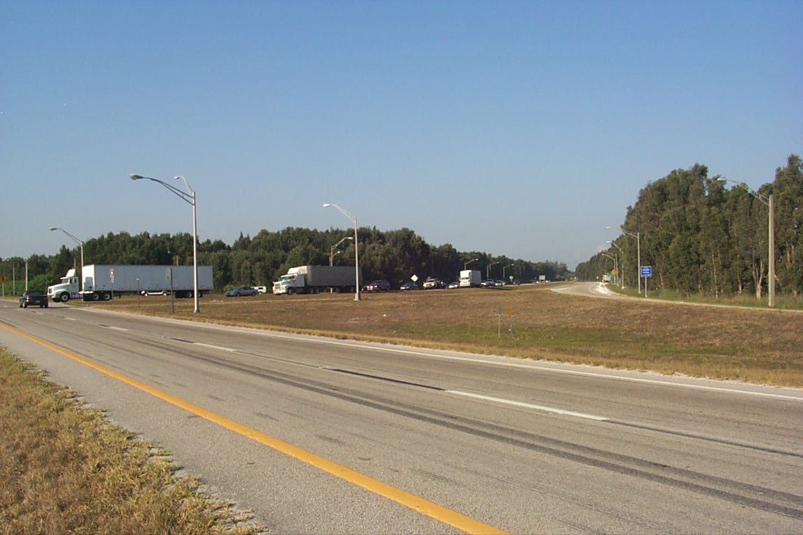
[ Back ] to Problem 3 [ Continue ] with Sub-Problem 4a

Sub-problem 4a: Potential Left-Turn Capacity

Step 1. Setup

Exhibit 3-26 shows the northbound left-turn queue at the Okeechobee Road Intersection. Observe the number of heavy vehicles in the traffic stream.

The heavy northbound congestion evident in the current operation (see Exhibit 3-26) suggests that the capacity of the northbound left turn should first be examined by the basic principles set forth in the HCM before the full procedure is invoked by software. This step will give us a better understanding of the basic relationships that apply to TWSC control.

Consider:

• What volume-related factors affect the northbound left-turn movement capacity?

• What geometry-related factors affect the northbound left-turn movement capacity?

• How could we take into account the separation of the roadways?

Discussion:
Take a few minutes to consider these questions. Click continue when you are ready to proceed.

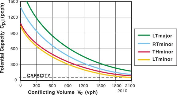
[ Back ] to Problem 4 [ Continue ] with Sub-Problem 4a

Sub-problem 4a: Northbound Left-Turn Capacity

Step 2: Results

What volume-related factors affect the northbound left-turn movement capacity? The basic relationship between movement capacity is defined by the conflicting flow rate and the driver characteristics (critical gap and follow-up time). Using what are widely considered default values for critical gap and follow up time as described in HCM Exhibit 17-5, one can graphically represent the relationship as shown below (which is similar to HCM Exhibit 17-7). This exhibit shows how the capacity for the stopped movement decreases as the conflicting volume (flow ratio on the x axis) increases. At very high levels of conflicting traffic, the capacity for the stopped movement becomes effectively zero because the availability of acceptable gaps is eliminated.

What geometry-related factors affect the northbound left-turn movement capacity? How could we take into account the separation of the roadways? A review of the aerial shows that the median space provides a potential refuge for vehicles that use two-stage gap acceptance. The right-turning traffic is removed from the intersection. Thus, consideration of the northbound left-turn movement becomes the eastbound through traffic as the only opposing movement in consideration of the first part of the two stage movement. The analysis that follows considers the first stage in consideration of the capacity of the northbound Krome Avenue left-turn movement. It should be noted that this is a simplification and may not consider the operation of vehicles in the median blocking northbound left-turn traffic from initiating this first stage of the two-stage gap acceptance. In this example, it is clear that the primary conflict under these traffic conditions is the eastbound through movement which is significantly higher than the westbound through movement.

[ Back ] [ Continue ] with Sub-Problem 4a

Sub-problem 4a: Northbound Left-Turn Capacity

Exhibit 3-27 shows several lines plotted on this exhibit which represent different types of stopped movements (through, left, etc.). The dashed red line has been added to identify the relationship for the minor street northbound left-turn movement. The westbound left-turn movement (solid black line) represents the potential capacity for the major street left turn, which must yield to the oncoming eastbound traffic and has a higher capacity than the movements entering from the minor street.

The dotted blue lines near the bottom of the graph represent the demand volume (Volume) and the estimated potential capacity (Capacity) based on the conflicting volume for the northbound left-turn movement.

[ Back ] [ Continue ] with Sub-Problem 4a

Sub-problem 4a: Northbound Left-Turn Capacity

The logical conclusion to draw from the graph on the preceding page is that the minor street conflicting movement volume is too heavy to permit a viable TWSC operation at this intersection. Without going into the numbers, the graphical presentation indicates that the demand volume is considerably higher than the capacity. Keeping in mind that the potential capacity for a movement does not consider the competition from other movements at the same priority level, it will generally represent an optimistic assessment of the capacity. When even this optimistic assessment fails, you would conclude that there is no point in proceeding any further with the investigation of TWSC.

Normally you would stop at this point and look at some other control alternatives. We will, however, carry the TWSC concept into a couple of other sub-problems to illustrate some features of the HCM analysis procedure and to set the stage for the consideration of other alternatives.

[ Back ] [ Continue ] to Sub-Problem 4b

Sub-problem 4b: Two-way Stop Controlled Analysis

Step 1. Setup

The unusual geometrics, especially the physical distance separating the conflicting movements at this intersection, will require some thought about how to represent the intersection for analysis by the HCM procedures. The conventional intersection conflict points are shown in Exhibit 3-28. Because of the wide separation of conflicts at this intersection, it should occur to us that we probably shouldn’t treat this situation as a typical urban intersection.

In this sub-problem, we will carry out a conventional intersection analysis. Then we will examine the results to determine if our treatment was appropriate.

Consider:

• What movements are considered in the HCM procedures?

• What is the basis for determining LOS in the unsignalized intersections methodology?

Discussion:
Take a few minutes to consider these questions. Click continue when you are ready to proceed.

[ Back ] to Sub-Problem 4a [ Continue ] with Sub-Problem 4b

Sub-problem 4b: Two-way Stop Controlled Analysis

What movements are considered in the HCM procedures? The HCM procedures compute the capacity, control delay, and level of service for all movements that must yield to other movements, including the left turns from the major street. Through and right-turn movements on the major street are excluded from the analysis and are assumed to have no delay.

This simplifying assumption raises a point of interest. Heavy vehicles making right turns will sometimes cause significant delays to traffic on the major street. This phenomenon is overlooked by the HCM procedure. If such delays are of concern to a particular analysis, it will be necessary to apply microscopic simulation modeling tools to supplement the HCM analysis. For purposes of this discussion, we will assume that traffic delay to the through movements on the major street is not an issue.

What is the basis for determining LOS in the unsignalized intersections methodology? The level of service is based on the control delay according to Exhibit 3-29. HCM Chapter 17 prescribes the full procedure for computing control delay.

[ Back ] [ Continue ] with Sub-Problem 4b

Sub-problem 4b: Two-way Stop Controlled Analysis

Step 2. Results

The results of this analysis are presented in Exhibit 3-30. These results reaffirm the conclusions drawn from sub-problem 4a, specifically that TWSC is not a viable control alternative. The v/c ratio for the NBL movement was 3.72, i.e., the volume was 372% of the capacity. The NBR movement v/c ratio was 1.92.

The WBL movement, on the other hand, appears to be operating within its capacity, with a v/c ratio of 0.71. This presents an interesting contrast with the NBL movement, since both movements have to contend with the same conflicting volume (i.e., 2,010 vph from the WBT). The difference may be seen in both the graphical representation of Exhibit 3-27 and the numerical presentation on Exhibit 3-. In the graph, the line representing the WBL shows a much higher capacity for a given level of opposing volume than the line representing the NBL movement.

[ Back ] [ Continue ] with Sub-Problem 4b

Sub-problem 4b: Two-way Stop Control with a Normal Urban Intersection Treatment

Exhibit 3-30 explains why these lines are in different places. The formula for computing the capacity of a movement that must yield to an opposing movement is given in HCM equation 17-3. This equation contains two parameters:

1. The critical gap, which indicates the length of a gap in the opposing flow required to accommodate the first queued vehicle trying to cross the opposing flow.

2. The follow-up time, which indicates the additional gap length required to accommodate each subsequent vehicle entering the same gap in the opposing traffic.

Larger values for each of these parameters will lower the capacity for the entering movement. The values shown in Exhibit 3-30 indicate lower values for the left turn crossing the opposing traffic than for the minor street entry movements. This indicates that drivers making left turns from the major street are willing to accept shorter gaps in the opposing traffic than drivers that are entering the major street from a minor street approach. The result is a higher capacity for the WBL movement compared to the NBL movement.

One of the objectives of this exercise was to judge whether it is appropriate to consider the intersection in the context of a normal urban intersection with TWSC control. This task can be accomplished best by comparing the results in Exhibit 3-30 with the corresponding results obtained by treating each of the conflict points separately. We will examine the separation of conflict points in the next sub-problem.

[ Back ] [ Continue ] to Sub-Problem 4c

Sub-problem 4b: Off-Peak Operational Analysis of Alternate Route 7

Step 2. Results

Let's first consider the level of service for the facility, or, more correctly, for each section of the facility that makes up this analysis. We need to note that, using this method, there is no overall performance measure for the facility as a whole. Part 3 of the HCM does cover issues relating to corridor and area-wide analysis. But we will not cover them here. If you are interested in learning more about this topic, consult part 3 of the HCM.

The level of service for each section is shown in the table below. Each of the sections performs at level of service C or better, with the exception of section 2, the weaving section. This result is consistent with our analysis produced in Problem 2 where we identified deficiencies with this weaving section during the peak period. We also noted that, while speeds in other sections are nearly 50 mph or above, section 2 has a forecasted speed below 28 mph, indicating a problem in the performance of the weaving section.

We can also note that the demand/capacity ratio is near one for this section. What is the implication of a demand/capacity ratio that is this high?

[ Back ] [ Continue ] with Sub-problem 4b 

Sub-problem 4b: Off-Peak Operational Analysis of Alternate Route 7

When we examine the part of the performance table (see below) dealing with ramp operations, we can see one of the results of the d/c ratio near one for the weaving section (section 02). Both the demands on the on and off-ramps are not completely served during this time period. Note for example that the demand for the on-ramp is 2,835 vehicles, while the actual ramp volume is 2,100 vehicles. But there are two points to make here that limit the applicability of these results. First, a limitation in the software used to implement the HCM did not allow entry of 2 lanes to the on-ramp. This produces an unreasonable result of ramp delay and queuing. Second, if this limitation was not present and the results were as shown in the table, the unserved demand during this time period would be transferred to the next 15-minute time period. The same caveat must be applied to the off-ramp results. So, while we can learn an important point about oversaturated conditions (demand exceeds capacity), this example does have a limitation (due to the software) that we need to keep in mind. [*team members: do we want to include a result like this in the guide?*]

These results apply to the off-peak period. In sub-problem 4c, we will consider the peak hour operation of the facility.

 [ Back ] [ Continue ] with Sub-problem 4b 

Sub-problem 4c: Separating the Conflict Points for TWSC Control

Step 1. Setup

Because of the wide median and the high speed rural type channelization of the right turns, it could be argued that the Okeechobee road intersection is likely to operate not as the single urban intersection considered in sub-problem 4a but as four separate intersections, with each intersection representing one of the conflict points, as shown in the diagram at the right. The separation of conflict points will usually give a more optimistic assessment of the operation than will the aggregation of conflict points into a single intersection. 

Consider:

• Why would separating conflicts produce a more optimistic assessment of the intersections?

• How are the conflict points inter-related?

Discussion:
Take a few minutes to consider these questions.  Click continue when you are ready to proceed.

[ Back ] to Sub-problem 4b [ Continue ] with Sub-Problem 4c

Sub-problem 4c: Separating the Conflict Points for TWSC Control

Let's consider the questions from the previous page.

Why would separating conflicts produce a more optimistic assessment of the intersections?  Separating conflicts may produce a more optimistic assessment, because as conflicting streams of traffic are removed from consideration, it results in more opportunities for acceptable gaps. The relationship is exponential and depending on conditions that may result in significant overestimation of capacity. For this reason, caution must be used when separating the conflict points for an unsignalized intersection.

How are the conflict points inter-related?  The most obvious relationship between the conflict points is how the paths of vehicles overlap multiple conflict points. For example, the northbound left-turn movement must pass through two points. Thus, if the second conflict path (northbound left turn and westbound through) is currently blocked by a queue of vehicles waiting for access, the analysis may be invalid. To determine whether the conflict points at an intersection may be separated, it is necessary to estimate the queue length for the each of the entering movements. If the estimated queue lengths are greater than the available storage space, then the separation of conflict points may overestimate or produce an unrealistic assessment of the operation.

Step 2. Results

Exhibit 3-31 shows the results of this analysis. In all cases, the movement capacities were improved in comparison with Sub-problem 4b, which considered all of the intersection conflicts simultaneously. This would be expected, but the important question is whether or not the queue backup would exceed the available storage space, thereby invalidating the analysis. Inspection of Exhibit 3-31 indicates that the 95^th-percentile queue lengths remained well within the storage boundaries. So, it could be concluded that it is appropriate to separate the conflict points for this intersection. While the separation of conflict points improved the operation slightly, some of the movements remain badly oversaturated—and the earlier conclusion that TWSC will result in a peak hour deficiency is confirmed.

[ Back ] [ Continue ] with Sub-Problem 4c

Sub-problem 4c: Separating the Conflict Points for TWSC Control

One more observation may be made from Exhibit 3-31. The NB right turn, even with the conflict points separated, indicates an oversaturated condition when analyzed as a TWSC operation. Because of the geometrics, the right-turn entry has more of the characteristics of a merge than a stop-controlled approach. This should raise some question as to whether another analysis procedure might be more appropriate. The treatment as a freeway entrance ramp will be considered in the next sub-problem.

[ Back ] [ Continue ] to Sub-Problem 4d

Sub-problem 4c: Peak Operational Analysis of Alternate Route 7

Let's now consider time period 2, the second 15-minute period during the PM peak period. The results for time period 2 are shown in the table below. Study the data presented in the table carefully.

Discussion:
As you review the data in the table above, what differences do you see between these results and those from time period 1? What is the most important information you learn from this table? When you are ready, proceed to the next page.

[Back] [Continue] with Sub-problem 4c 

Home > Problem 4 > Sub-problem 4c - Page 5 of 7

Sub-problem 4c: Peak Operational Analysis of Alternate Route 7

The main point that we can learn from the table showing results from time period 2 is that we have a bottleneck, a point along the freeway facility that limits or constrains the demand. This bottleneck shows up in section 6, where the volume/capacity ratio equals one.

What is the cause of this constraint? If we review the line drawings showing the geometric information for the eastbound portion of Alternate Route 7, we see that this is where the mainline drops from three lanes to two lanes. At this point, the demand exceeds the capacity of the two lane section and a queue begins to build at this point, traveling upstream. At the end of this 15-minute period (time period 2), the queue extends the entire length of section 5 (1,890 feet). It also reaches section 4 nine minutes after the beginning of time period 2 and extends 745 feet through this section by the end of the 15-minute time period.

Both sections operate at level of service F, even though the demand/capacity ratios for these sections are well below 1.0. Why? These sections are in the congested regions of the speed/flow diagram (*add link*), as shown by the very low speeds (below 30 mph) that exist in these sections.

[Back] [Continue] with Sub-problem 4c 

Home > Problem 4 > Sub-problem 4c - Page 6 of 7

Sub-problem 4c: Peak Operational Analysis of Alternate Route 7

Let's note one other result for the sections downstream from the bottleneck (section 6). Note that the volume/capacity ratio is less than the demand/capacity ratio. Or, similarly, the demand is higher than the volume. What is the implication of this result? Some vehicles that desire to reach sections downstream from the bottleneck (sections 7 through 11) are unable to do so during time period 2. They are in the queue forming in sections 4 and 5 and will be delayed in this queue until at least time period 3. This unserved demand is transferred from time period 2 to time period 3.

When you are ready to review the results from time periods 3 and 4, proceed to the next page.

[Back] [Continue] with Sub-problem 4c 

Sub-problem 4c: Peak Operational Analysis of Alternate Route 7

The tables below show the results for time periods 3 and 4. We note in the first table that the queue formed during time period 2 clears during time period 3, by the first minute in section 3 and by the third minute in section 5. You can see that the demand that wasn't served during time period 2 has been transferred to time period 3, since the volumes in sections 4 through 11 that actually use the facility exceed the original demand for these sections. For example, in section 5, the volume is 1,745, while the demand is 1,270. This means that a flow rate of 1,745 minus 1,270, or 475, has been transferred from time period 2 to time period 3. And since the demand for time period 3 is low enough, there is sufficient capacity to serve both the original demand (1,270), plus the transferred demand (475).

During time period 3, all sections operate at level of service C or better, with the exception of section 5, which is still recovering from the queue, and operates at level of service E. The speed in section 5 is less than 20 mph during this recovery.

But by time period 4, all sections of the freeway facility are operating at LOS B or better. All speeds exceed 40 mi/hr. And, once again, the demand equals the volume, indicating that all vehicles desiring to travel along the facility during time period 4 are served.

[Back] [Continue] with Analysis

Problem 4: Analysis

We have now completed a review of the operation of Alternate Route 7 during the PM peak period. The operation of this facility is typical of many urban freeways during peak periods. At the beginning of the peak, the facility operates at acceptable levels of service, and all demand is served during the first 15-minute time period. During the second time period, a queue begins to form as the demand exceeds the capacity where the facility drops from three lanes to two. This is a classic freeway bottleneck condition. The queue extends from the bottleneck point between sections 5 and 6 (where the lane drop occurs) upstream through section 5 and into part of section 4. The bottleneck, and the resulting queue, delays vehicles that entered the system during time period 2 to the next time period. The queue clears during time period 3, and the freeway is back to good operation during time period 4.

The table below provides a summary of some of the key data for the four time periods that we have reviewed.

These summary data provide several interesting insights, at a more system level, on the performance of the freeway facility.

• Even in time period 1, when there is no queuing, there is delay. How can this be true? Recall that delay is the time that a driver spends traveling at less than preferred speed. The average mainline speed is less than 55 mph (54.42 mph), so there is some, though minimal, delay. The delay increases during time period 2 to nearly 1.5 minutes per vehicle, and the average speed drops to 44.15 mph.

• These system measures do provide a broad perspective on the performance of the freeway facility and are therefore valuable aids to analysts and decision makers. However, to understand the specific causes of delay or queuing, we must always look at the details of the facility performance, checking the data for each section to understand the causes of poor performance.

What are the implications of these results? Do we need to continue with further analysis of this freeway facility? When you are ready, proceed to the next page.

[Back] to Sub-problem 4c [Continue] to Discussion of Problem 4

Problem 4: Discussion

The freeway facility methodology from chapter 22 of the HCM has provided us with important insights on the performance of Alternate Route 7 during both the off peak and peak periods. We found the facility performs well during the off peak, but the lane drop from three to two lanes on the eastbound portion of the facility results in some delay for motorists during the PM peak period.

We also need to consider whether further analyses should be conducted to have a complete picture of the operation of this facility. Let's consider the following issues:

• Have we considered a wide enough view of the system?

• Are there limitations of the HCM methodology that require us to use other tools, such as simulation?

The system that we considered is the mainline portion of Alternate Route 7 from the I-87 interchange on the west to the I-787 interchange on the east. But do we need to extend the boundary of our study area further in order to capture any other effects? We know that there are problems with the interchanges themselves. Some of these problems appeared in the analysis that we conducted for problems 2 and 3 of this case study. So, widening the system to include the interchanges might prove beneficial in our assessment of Alternate Route 7.

This leads to the next issue, the possible use of micro-simulation. Under what conditions should we consider micro-simulation modeling? The first such condition is when demand exceeds capacity, particularly when there is an intersection of queues on the facility. Here, there is value in the ability of a micro-simulation model to follow the behavior of individual vehicles and drivers as they negotiate a congested facility. A second such condition is when we are considering a large and complex system, such as a freeway mainline and interchanges.

In problem 5 of this case study, we will illustrate how one micro-simulation tool can be used to study the operation of Alternate Route 7.

[ Back ] to Analysis of Problem 4 [ Continue ] to Problem 5