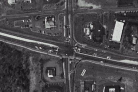
Problem 4: Clifton Country Road

Problem 4 Printable Version

The intersection of Clifton Country Road and Route 146 (Intersection D) is the most complex, busiest, largest, and most complex in the network. Exhibit 2-36 shows an aerial photograph of the site. (North is toward the top.)

The main question at this intersection will be: are geometric changes and/or adjustments in signal timing needed to accommodate the site-generated traffic? Since a lot of the site-generated traffic will be going to and from I-87, the signal timings will have to change, dictated by the actuated controller. But geometric changes might be needed as well. In the process of answering these questions, we can use this intersection to illustrate a number of analysis issues.

As you can see in Exhibit 2-37, the intersection’s eastbound approach is five lanes wide (left, triple through, and signalized right). The westbound approach is also five lanes wide (double left, double through, and free right). The southbound approach has three lanes (left, left/through, and right/through) while the northbound approach has four (double left, through, and free right). The eastbound left-turn bay is about 150 feet long. The westbound left-turn bay is about 400 feet long so it can accommodate heavy volumes coming from I-87. On the southbound approach, there’s space to store about 10 cars per lane to the upstream intersection with Old Route 146. On the northbound approach, about 20 cars can be stored per lane prior to the first side road intersection.

Problem 4: Clifton Country Road

As you can tell from the overview of the network we presented in the introduction, there are large shopping plazas both north and south of the intersection.  The road to the north ends in a shopping center parking lot while the one to the south threads its way between the Clifton Park Center shopping mall on the east and the Shopper’s World shopping center on the west.

About a tenth of a mile east of the intersection is the freeway interchange with I-87. That location will be the focal point of Problem 5. To the west is the Maxell Drive intersection that was the focal point of Problem 1.

Base Case Phasing and Volumes

Analysis Plans Description of Analyses

Overarching Issues

Sub-problem 4a: AM peak hour - Existing Conditions

Sub-problem 4b: PM peak hour - Existing Conditions

Sub-problem 4c: 2004 PM - With vs Without Conditions

Discussion

Discussion:
This is a complicated intersection. The challenge is to be clear about how the intersection is being represented in the analysis and be careful about interpreting the results. Primarily, the lane configurations and lane utilization make the analysis a challenge.

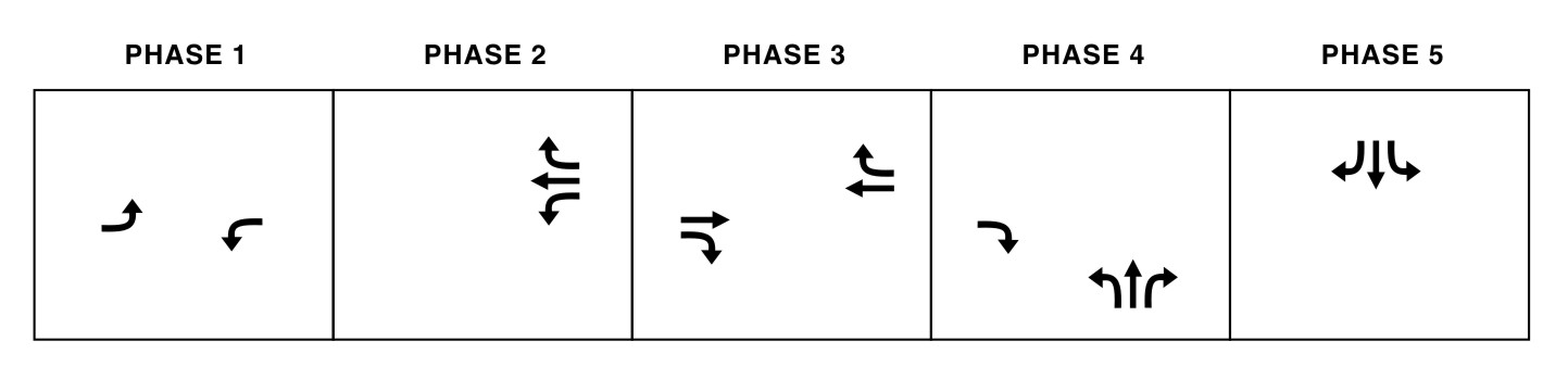
Problem 4: Clifton Country Road

Base Case Phasing and Volumes

The signal control is fully-actuated. Exhibit 2-38 shows the phasing. Phases 1-3 are for the east-west flows. The first phase is often skipped because the eastbound left turning volumes are small. Phases 4-5 are for the north-south movements except that Phase 4 has a protected green for the eastbound right.

Problem 4: Clifton Country Road 

Analysis Plans
As we illustrate the traffic impact assessment, we will explore a number of issues at this intersection, as Exhibit 2-3 indicated in the introduction. The intersection lends itself to consideration of time periods, relationships among HCM methodologies, consideration of times to use other tools, interpretation of results, etc. As we found with the Moe Road analysis, lane utilization will again be important in the context of the AM Existing conditions. In addition, we’re going to talk about general modeling issues such as lane groups, lost time, time periods to analyze, and chapter relationships. We'll also focus on the AM Existing condition and look at lane utilization, coordination, and lane grouping. For the PM Existing condition we will examine queue spillback, right-turns-on-red, and demand versus volume.  Finally, we’ll look at the PM With condition and analyze our assumptions about future conditions, geometric changes, and feedback.

to Overarching Issues

Problem 4: Clifton Country Road 

Overarching Issues
Several overarching issues relate to this intersection. There are some things to discuss before turning to the main purpose of the case study: seeing how to mitigate the impacts from the site-generated traffic.

The first relates to how many time periods we should analyze. That is, what time periods should be considered in examining the intersection’s performance? The answer is several. Clearly, the AM and PM peak hours should be examined. The intersection is part of a major east-west arterial, next to a major freeway interchange. However, the Saturday shopping peak should be examined as well. The intersection is adjacent to three major shopping centers.

We also need to think about whether there’s a peak hour of the generator that’s different from all three time periods, or a peak traffic condition that relates to this specific intersection. For example, we might want to examine the conditions on a Friday afternoon peak hour when the shopping volumes are heavier than they are during the rest of the week. Moreover, we might want to do a separate analysis of the intersection for the Friday afternoon and Saturday midday conditions during the November-December holiday shopping season. The three adjacent shopping centers see a significant growth in patronage during that timeframe. In fact, queues for the westbound left turn can reach as far as the bridges under I-87. The intersection shouldn't necessarily be designed to accommodate these relatively rare events, but it might be appropriate to indicate what the performance is like during these time periods and how many hours during the year the intersection will be in this condition.

This intersection is somewhat difficult to analyze in an isolated fashion, and care is needed. The most important reason is that there are queues on the southbound, northbound, and westbound approaches that can spill back into other facilities. We will analyze those facilities along with the Clifton Country Road intersection to make sure that we’ve taken into account the impacts in the results we present.

Problem 4: Clifton Country Road 

To treat the problem in this more systematic manner, we need to do an unsignalized intersection analysis at the two-way stop controlled intersection just to the north (visible in the aerial photograph). We will also do an analysis of the all-way stop controlled intersection beyond. We will also look at the two-way stop controlled intersection to the south. This means doing analyses based on Chapter 16 and Chapter 17 simultaneously.

In doing this, we also have to be careful to account for evidence of modifications to typical driver behavior. For example, when the westbound left-turn bays get congested, drivers that want to go south turn right instead, go north to the TWSC intersection at Old Route 146, then make a U-turn to again be headed south. They know the southbound approach will get a green before the next time the westbound left turn does. This action adds traffic to the Old Route 146 intersection and lengthens the queue on the southbound approach.

This discussion demonstrates the intersection may require other analysis methods. We may consider using a network analysis package that can simultaneously look at the performance of all the intersections we’ve discussed.

Discussion:
We return to the same discussion format used initially in the case study. We revisit the basic issues to identify the problem, how it should be approached, how large the study network should be, and what analysis tools need to be employed. Do you have facilities that are similar, where the general issue decisions you made for the overall problem need to be revisited and refined to address a more site-specific problem?

Sub-problem 4a: Clifton Country Road AM peak hour - Existing Conditions

The AM Existing conditions are well suited for looking at three issues: lane utilization, coordination, and lane group definitions. These issues have to be considered in all the other time periods as well. We will use the AM Existing condition to provide numerical results.

Analyses:

Lane Utilization

Coordination

Lane Group Definitions

Sub-problem 4a: Clifton Country Road AM peak hour - Existing Conditions

Lane Utilization
Lane utilization is an important issue on all four approaches. In the case of the eastbound approach, the I-87 southbound on-ramp is immediately downstream of the intersection. The right-hand-most through lane is used far more than the other two. There’s a secondary impact for drivers wanting to turn right who can’t get into the auxiliary right-turn lane because the long queue blocks access. For the westbound approach, the double left has unbalanced lane use. The innermost lane is sometimes blocked by the outer one. Traffic tends to use the outer lane because it leads to the Shoppers World Plaza and some convenience stores. In the case of the northbound approach, the double left has balanced lane use. The right-most lane leads to stores on the north side of Route 146 just west of the intersection, but there are also drivers who want to continue west, so both lanes see substantial use. For the southbound approach, the lane use is not necessarily unbalanced, but the lane use designations are complex (left, left/through, and through/right). We will study that approach separately.

Exhibit 2-40 shows the differences between including and not including lane utilization. The utilization values employed by movement are shown in the bottom line of the table. In Dataset 32 (the base case) and Dataset 33 (no lane utilization) the impact is substantial for the eastbound throughs. With the lane utilization included, that movement has a delay of 28.6 seconds per vehicle. Without it, the delay is only 22.5 seconds per vehicle, a 27% difference.

*Using an 82-second cycle length during the a.m. peak hour

Sub-problem 4a - Clifton Country Road AM peak hour - Existing Conditions

Coordination
Since this intersection is part of a network, we must determine whether coordination would be useful for the eastbound approach. The westbound approach has traffic coming from both southbound and northbound off-ramps as well as Route 146, so coordination wouldn’t be as useful there.

Sub-problem 4a: Clifton Country Road AM peak hour - Existing Conditions

Lane Group Definitions

In most analyses, it’s easy to correctly define the lane groups. In the case of Moe Road, for example, there are left-turn lanes, through lanes, and through-and-right lanes. On the eastbound and westbound approaches, we considered the through lane and the through-and-right lane to be a two-lane through-and-right group. In these latter situations, we assume that 1) the right turning vehicles are in the right-most lane and 2) the through traffic distributes itself between the right-most lane and the next inner lane to balance the per-lane flow rates.

The HCM is capable of analyzing many different lane groupings: exclusive lefts (one, two, three, etc. lanes), shared left-and-through lanes, through lanes, shared right-and-through lanes, exclusive rights, etc. But it cannot do lane-by-lane analyses, and there are some lane groups that it doesn’t accommodate easily. One of those is the southbound approach.

The southbound approach has the following lane configuration: left, left/through, and through/right. The HCM doesn’t provide for an exclusive left-turn lane in conjunction with a left/through lane. That means you have to decide how this approach should be modeled. Two criteria must be satisfied. First, the innermost lane gets as much use as the center lane and the outermost lane gets very little use. Second, the queue lengths on the innermost lane and center lane are about balanced.

We compared and contrasted three ways to represent the southbound approach. In Dataset 32, the base case, which we prefer, we assume the innermost lanes are used only for left turns, and the outermost lane is used for throughs and rights, shown as the first condition in Exhibit 2-42. This simplification is not a major misrepresentation of the way the approach works, but it is a simplification. There are through vehicles that use the middle lane. That option produces equal delays for the lefts and the throughs and rights, and the queue length estimates (average and 95^th percentile) for the left-turning lanes are double those of the through-and-right lane. That is consistent with the field observations.

Sub-problem 4a: Clifton Country Road AM peak hour - Existing Conditions

*Using an 82.0 second cycle length during the a.m. peak hour

You can also group all the movements together and have a generic 3-lane approach (Dataset 36). That produces the Single SB Group results shown in Exhibit 2-42. The results aren’t significantly different from those in the base case, but the distinction is lost between the innermost two lanes and the outer lane.

You could also create a scenario that looks like field observations: a single left-turn lane, two lanes assigned partially to through movements, and shared lefts and rights (Dataset 37). However, this produces a result that is very different from the base case, as seen in the third scenario in the table. The delays for the southbound left are quite large, 49.9 seconds per vehicle, and the queue length values are two-and-a-half times those of the base case. This lane grouping definition doesn’t match the field conditions.

We have identified a way to model the situation that matches the behavior that’s been observed in the field. In this case, the base case or the single SB lane group seems best.

Sub-problem 4b: Clifton Country Road PM peak hour - Existing Conditions

Analyses:

Lost Time

Demand vs. Volume

Right Turns On Red

Sub-problem 4b: Clifton Country Road PM peak hour - Existing Conditions

Lost Time
Start-up lost time is the seconds of green that go unutilized because it takes the lead vehicles a little while to get going. The HCM default is 2 seconds. Sometimes, the intersection geometry lengthens this figure. In this case, the northbound and southbound approaches have a slightly longer lost time, because of an upgrade and the geometry of the left-turn moves. It takes the discharging queues a short while to get organized before vehicles start to flow smoothly. Increasing the start-up lost time to 3 seconds, which is what we’ve assumed, lets us account for the delay due to the slope.

At the end of the green, you also have to specify the extension of effective green. This is the number of seconds, after the light goes yellow, that vehicles are still entering the intersection. The HCM assumes 2 seconds. The HCM's default assumptions, then, are that the specified green time is the same as the length of the effective green time. The ideas are different, but the numbers are the same. If you have a green 20 seconds long, and a yellow that’s 3 seconds long, then the lost start-up time means that vehicles are moving during only 18 of the 20 seconds of green, losing 2 seconds. On the other hand, if you assume a green time extension of 2 seconds, vehicles are still entering the intersection for 2 of the 3 seconds of yellow, gaining the two seconds of lost time.

By assuming the start-up lost time is 3 seconds and leaving the extension of green unchanged at 2 seconds, we assume the amount of effective green available to the northbound and southbound flows is one second shorter than the green time we assign. If the green time is 20 seconds, subtracting 3 and adding back 2 means we have 19 seconds of effective green.

Sub-problem 4b: Clifton Country Road PM peak hour - Existing Conditions

Demand vs. Volume
When you collect turning movement counts at an intersection, you are recording the output from the intersection, but not necessarily the input. Traffic counts record the vehicles that have been processed by the intersection, leaving uncounted those that are queued up and waiting to be processed. The counts you collect are volumes, and the arrivals are demand. In many cases, congested intersections have demand/volume ratios greater than 1.0 during the peak hour. That is, the arriving demands are greater than the intersection can handle. Queues begin to form and grow while the demand to capacity (D/C) ratio is greater than 1.0. They only begin to dissipate when the D/C ratio becomes less than 1.0.

Sub-problem 4b: Clifton Country Road PM peak hour - Existing Conditions

Right Turns on Red
In all of the datasets for the Clifton Country Road intersection we assumed there are a substantial right turns on red (RTOR) for the eastbound, westbound, and northbound approaches. (click here to open any one of the datasets.) Each of these three approaches has an auxiliary right turn lane. The one difference among them is that the eastbound right-turn lane is quite short and the right turn on red is often difficult to make because the lane is blocked, the westbound lefts are turning, or the southbound throughs are in motion.

Exhibit 2-44 shows you the difference in predicted performance between the base case PM Existing condition and condition where the RTOR on the eastbound, westbound and southbound approaches are prohibited.  Follow the link to see Dataset 38 (2002 PM base case) or Dataset 39 (RTOR prohibited) datasets. In the base case, 10% of the eastbound rights turn right on red. For the westbound approach, all of the right turns are omitted because there is a separate right-turn auxiliary lane and there isn’t much opposing traffic. For the northbound approach, as many vehicles turn right during phases 1 and 2 as westbound lefts in a single lane (550/2). Another 10% of the northbound rights move during other times when the light is red northbound. Southbound, there are no right turns on red. In the RTOR prohibited dataset, all the right-turn-on-red volumes are set to zero except for the northbound approach where the volume is set to 275, reflecting the number of right turns that move when the westbound left is moving.

Notice that the eastbound and westbound RTOR values can be zero and the intersection can still function well. Neither of these RTOR prohibitions causes a catastrophic increase in delay. The eastbound right-turn delay grows from 14.0 to 14.5 seconds per vehicle. The westbound delay grows from 13.1 to 16.3 seconds per vehicle. The base case assumes that these auxiliary lanes are reachable, meaning that the length of the eastbound lane must be 10-20 cars long to be reachable 50-95% of the time, and the westbound lane must be 10-19 cars long.

For the northbound approach, a RTOR prohibition creates LOS F (these results are not shown in the table.)  In fact, the smallest feasible RTOR value is 297 vehicles. That is, if the RTOR value was decreased from the base case, through some traffic engineering treatment, the smallest it could be would be 297 vph and still have LOS F for the northbound rights.

Sub-problem 4b: Clifton Country Road PM peak hour - Existing Conditions

Notice that we can drop the eastbound and westbound RTOR values to zero and the intersection still functions well. Neither of these right turns has catastrophic increases in delay. The eastbound right-turn delay grows from 14.0 to 14.5 seconds per vehicle. The westbound delay grows from 13.1 to 16.3 seconds per vehicle. The base case assumes that these auxiliary lanes are reachable, meaning that the length of the eastbound lane must be 10-20 cars long to be reachable 50-95% of the time, and the westbound lane must be 10-19 cars long.

For the northbound approach, however, the RTOR value cannot drop to zero without creating LOS F. In fact, the smallest feasible RTOR value is 297 vehicles. That means, of the 508 northbound right turns, 58% (297/508) must be able to make a RTOR to make the intersection work. The intersection currently operates this way; no standing queue exists in that lane.

Sub-problem 4c: Clifton Country Road 2004 PM - With vs. Without Conditions

It’s in the comparison of the with versus without conditions for the future design year, the traffic impact assessment finds its main emphasis. What network enhancements are required to accommodate the without conditions? Nominally, those improvements are the responsibility of the owning and operating agency. The differences between the without and the with condition are traceable to the development.

Sub-problem 4c: Clifton Country Road 2004 PM - With vs. Without Conditions

Without
In the PM Without condition, the interesting issue is the intersection’s performance. This situation sets the standard against which the PM With condition is compared. Exhibit 2-46 shows the performance of the intersection under four conditions: PM Without (Dataset 40); a PM With condition in which the site-generated flows are at their expected values (Dataset 41); a PM With condition in which the site-generated traffic is 30% greater than those expected values (Dataset 42); and a PM With condition in which intersection enhancements have been made to improve the facility’s performance (Dataset 43).

In the PM Without condition, the delays are substantial. They range from 13.7 to 62 seconds per vehicle, with many being above 50. The overall average delay is 56.2 seconds per vehicle. The average queue lengths are predominantly around 8-12 vehicles and the 95^th percentile queue lengths range up to 21 vehicles. Five of the v/c ratios are 0.80 or above.

With
The with condition makes the situation worse. Delays are higher (the average delay is higher by 5.5 seconds per vehicle), v/c ratios are higher, and queues are longer.

With Plus 30-Percent

We will explore the impacts even further by examining a situation where the site-generated traffic was 30% greater than projected. That scenario is presented third. One movement (the eastbound through) now has a v/c greater than 1.0, several movements are at LOS E, and the overall intersection level of delay is 51 seconds per vehicle.

Sub-problem 4c: Clifton Country Road 2004 PM - With vs. Without Conditions

Sub-problem 4c: Clifton Country Road 2004 PM - With vs. Without Conditions

Mitigation
The next question is: what can be done to mitigate this impact? Adding lanes is the usual solution. But at this intersection it would be difficult. Reconstruction would be expensive and disruptive, so we will explore other options. Look at Dataset 42 to see the analysis of the PM With condition plus 30% higher traffic and the poorer performance. Dataset 43 contains the analysis of the dataset in the enhanced condition.  The results from these two analysis are shown in Exhibit 2-46.

The differences derive from three sources. First, we assumed that coordination would be introduced for the eastbound flows. We changed the arrival type from 3 to 5 for the eastbound through and right.

We considered decreasing the unit extension from 3 seconds (the default) to 2, which the HCM predicts will reduce delays; but in the field, such reductions often produce premature phase terminations, which actually increase delay instead of decreasing it.

We also debated reducing the start-up lost time from 3.0 to 2.0 seconds for the northbound and southbound approaches but failed to see how the change could be defended without reconstructing the intersection.

We did consider increasing the cycle length beyond 108 seconds, but chose to reduce the cycle time instead. (See later text.)

The more substantial change was to the lane utilization coefficients. We assumed they were all at default values, because the site-generated traffic is going straight ahead (not onto I-87), so the lane utilization will be better than the condition originally observed in the field. The lower v/c ratio eastbound made it possible to remove green time from phase three and shorten the cycle length. It also made it possible to add time to phase 5. The end result is an intersection that is at LOS D or better for all movements, even under the 30% higher site-generated traffic conditions. This is a substantial improvement; and it illustrates the value of carefully organizing the flows, if possible.

Problem 4: Clifton Country Road

Discussion
This problem has explored a number of capacity modeling issues in the context of the Clifton Country Road intersection. Consistent with Exhibit 2-3, we examined time periods, the relationships among HCM methodologies, times to use other tools, interpretation of results, etc. As we found with the Moe Road analysis, lane utilization will again be important. We looked at that in the context of the AM Existing conditions. In addition, we examined lane groups and lost times. In the case of the PM Existing conditions, we explored issues of queue spillback, feasibility of identified solutions, demand versus volume, and right turns on red. In the PM With condition, we focused on feedback (in terms of design), the impacts of various assumptions about the future conditions, and the tie between geometric changes and intersection performance.  Only changes to the signal operation and lane utilization were explored.  No geometric changes explored.