Problem 3: Basic Freeway Sections

Printable Version

This problem is focused on the complex of interchanges located on the eastern end of Alternate Route 7. The main emphasis is on the interchange between Route 7 and I-787.

Exhibit 4-39 contains a diagrammatic picture of the interchange complex on the eastern end of Alternate Route 7. As can be seen, the Route-7/I-787 interchange is basically a cloverleaf with one semi-direct ramp. Originally, the plan was to have I-787 continue eastward, through Troy, and overlap the Route-7 alignment to the Vermont border. The idea was squelched when it became clear that the freeway alignment through Troy would involve taking many homes and effectively closing Hoosick Street, a major arterial.

Consistent with Table 1 in the introduction, Exhibit 4-39 also shows the locations where specific analyses will be focused:

1. Westbound weave on Route-7 as it crosses the Hudson River.

2. Eastbound weave on Route-7 as it crosses the Hudson River.

3. Northbound weave on I-787 between the 23^rd street interchange and the Route 7 interchange

4. Southbound weave on I-787 between the 23^rd street interchange and the Route 7 interchange

5. Northbound weave on I-787 between the loop ramps

6. Eastbound diverge on Route 7 that leads to both the right-hand ramp to I-787 and the auxiliary lane that connects to the loop ramps to and from I-787

7. Southbound merge between the right-hand ramp coming from Route 7 east and the semi-direct loop ramp coming from Route 7 west.

8. Southbound merge between the combined ramp from G above and I-787 south.

9. Westbound merge between Route 7 and the loop ramp coming from I-787 north.

10. Westbound merge between Route 7 and the right-hand ramp coming from I-787 south.

11. Eastbound merge between the auxiliary eastbound lane on Route 7 and the loop ramp coming from I-787 southbound.

12. Eastbound diverge involving the auxiliary eastbound lane on Route 7 and the loop ramp leading to I-787 northbound.

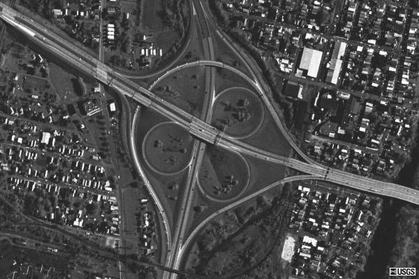
Problem 3: Basic Freeway Sections

Exhibit 4-40 contains an aerial photograph of the I-787 interchange. You can see the three loop ramps, the four right-hand ramps, and the semi-direct ramp leading from Route 7 westbound to I-787 southbound. You can also see the auxiliary lane on the south side of eastbound lanes that starts with the right-hand ramps extends through the two loop ramps and then reunites with the eastbound lanes just east of the east-to-north loop ramp. The figure also shows the short northbound weaving section under the Route 7 bridges and the tight radius that is part of the right-hand ramp leading from Route 7 eastbound to I-787 southbound.

Exhibit 4-40. Aerial Photograph of the I-787 Interchange

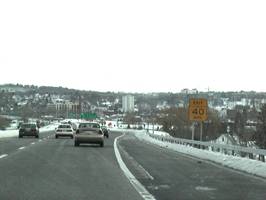
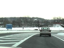
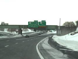
Problem 3: Basic Freeway Section

Exhibit 4-41 shows a view of Route 7 at location F looking eastbound toward Troy. You can see the beginning of the auxiliary lane that leads to the right-hand ramp and the loop ramps. In the background, you can see the signs for the loop ramp to I-787 north and the merge sign for the place where the auxiliary lane rejoins Route 7 east.

Exhibit 4-42 shows a view of location G where the right-hand ramp from Route 7 east to I-787 south merges with the semi-direct ramp coming from Route 7 west. You can see the semi-direct ramp from Route 7 east to the left of the vehicle ahead and you can tell that the two single lane ramps are about to merge not far downstream.

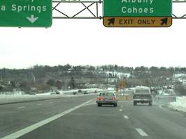
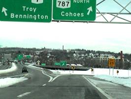
Problem 3: Basic Freeway Sections

Exhibit 4-43 shows a view of Location C looking north, just before the double-lane right-hand ramp leaves to head toward Route 7 east. You can see the two lanes of I-787 that continue north under the railroad bridge and then Route 7. You can also see the signs for Route 7 east on the right (leading toward Troy) and Route 7 west (leading toward Saratoga Springs). The truck in the distance at the front of the platoon traveling north on I-787 is at the beginning of the weaving section designated as Location E in Exhibit 4-39.

Exhibit 4-44 shows a view of Route 7 west just at the end of the weaving section designated as Location A in Exhibit 4-39. You can see the beginning of the semi-direct ramp leading from Route 7 west toward I-787 south. Just beyond the view in the picture is the point where the right-hand ramp to I-787 north branches off to the right. You can also see cars on Route 7 east and, if you study the photo very carefully, cars on the auxiliary lane that connects to the loop ramps to and from I-787. The loop ramp associated with Location I can just barely be seen in the distance, behind the sign with the two downward arrows between the car and the truck.

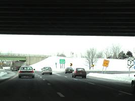
Problem 3: Basic Freeway Sections

Exhibit 4-45 shows a view of Location E looking north taken from a location that is about halfway through the weaving section at Location E. The sign to Route 7 west can be seen at the right-hand edge of the picture. The bridge immediately overhead is Route 7. The bridge in the background is the semi-direct ramp leading from Route 7 westbound to I-787 southbound. The merge sign in the distance at the left-hand edge of the picture is associated with the location where the right-hand ramp from Route 7 west merges with I-787 north.

Exhibit 4-46 shows a view looking east at Location L. The left-hand lane is the auxiliary lane that goes from Location F on the western end to a point just beyond Location L. To the left in the picture you can see the place where the auxiliary lane rejoins Route 7 east. The right-hand lane is simultaneously the end of the south-to-east loop ramp going from I-787 south to Route 7 east and the beginning of the east-to-north loop ramp going from Route 7 east to I-787 north. You can see the start of the east-to-north loop ramp in the right-hand side of the picture. In the distance, you can see the spot where the right-hand ramp from I-787 to Route 7 joins Route 7, which is also the start of the weaving section at Location B.

Sub-problem 3a: Weaving Segment A and B

Step 1. Setup

This sub-problem focuses on the six weaving sections in the Route 7/I-787 interchange. In Exhibit 4-39, they are at locations A, B, C, D, E, and between locations K and L. We’ll study each of these, to some degree. As you proceed through this sub-problem, think about:

Discussion:
Take a few minutes to consider these questions. Click continue when you are ready to proceed.

Sub-problem 3a: Weaving Analysis

When you’re studying a weaving section, it is important to consider 1) type of weave, 2) weaving length, 3) distribution of flows within the weave, 4) speeds of the weaving and non-weaving movements, 5) peak hour factor, 6) percentages of trucks, buses, and recreational vehicles, and 7) passenger car equivalents for each of these.

Weaving sections are type A, B, or C, depending on how many lane changes are required for the weaving movements. Page 13-13 in the HCM 2000 tells you how these weaving types are defined. A Type A weave involves at least one lane change for both weaving movements. If two freeways both enter and exit a weave, to get from one to the other, at least one lane change is required. In a Type B weave, one of the two weaving movements doesn’t have to change lanes and the other changes only one lane. In a Type C weave, one of the two weaving streams has to shift at least two lanes.

Another necessary fact is whether or not the weave is constrained. In general, vehicles have difficulty changing from one lane to another in a constrained weave; whereas, in an unconstrained one, they don’t. The same analysis must be conducted for both weaves to determine which condition pertains. That will be determined by the number of lanes required for the weave. The minimum number required for unconstrained operation varies by type of weave. For Type A weaves, 1.41 lanes are required. Consequently, if the formula says more than 1.41 lanes are required for the weave, the weave is constrained.

For weaving sections, level of service is determined by what the formulas predict is the density of vehicles (passenger cars per mile per lane, or pcpmpl). The formula requires the volumes in weaving traffic streams, the number of lanes in the weaving section, and the speeds for the weaving and non-weaving vehicles. You can read Chapter 13 in the HCM for a more complete discussion about how this performance measure is defined for weaving sections. The breakpoints for LOS are the same as for basic freeway sections.

Sub-problem 3a: Weaving Analysis

Step 2. Results

Weaving Segments A & B
The weaving sections at A and B may be the easiest to analyze, so we’ll study them simultaneously. Each is four lanes wide and approximately 3,100 feet and 2,600 feet in length, respectively. The entering and exiting facilities are both two lanes wide. Each weaving section is Type A, because the weaving vehicles on the upstream facility must make at least one lane change to complete the weave.

The field data upon which the methodology is based suggests that the weaving and non-weaving speeds are different from one another. To compute the weaving and non-weaving speeds, we need to do two calculations using equation 24-2 in the HCM 2000 to determine the average speed of the weaving, S_w and non-weaving vehicles, S_nw.

Sub-problem 3a: Weaving Analysis

As the weaving and non-weaving vehicle speed equation shows, these speeds depend on weaving and non-weaving intensity factors that measure the influence of the movements on the overall speed. The calculations of the weaving and non-weaving intensity factors, W_w and W_nw, respectively, use equation 24-4 in the HCM 2000.

The values for the various constants depend on the type of operation within the facility (constrained or unconstrained). These values were derived from a multi-variable, non-linear regression analysis of field data.

Sub-problem 3a: Weaving Analysis

The results of the calculations are show in Exhibit 4-47. The calculations suggest that both of these weaving sections have adequate levels of service in the AM and PM peaks.

Before concluding that these facilities are operating acceptably, we should note that the weaving sections are longer than the distances that the HCM 2000 methodologies were designed to address. The HCM 2000 says that if the weaving section is longer than 2,500 feet, it should be analyzed as a combination of an on-ramp and an off- ramp, which we did in Sub-problem 2b. For this problem, however, we analyze them if they were only 2,500 feet long, so we’re not outside the range for which the HCM is intended. That produces the results shown in Exhibit 4-47.

Notice that the weaving and non-weaving intensity factors, W_w and W_nw are higher when the volumes are higher. That means they’re higher in the AM peak for Location A and in the PM peak for Location B. This increases the densities and produces a lower level of service.

Sub-problem 3a: Weaving Analysis

Another thing to note is that the operation of these weaves is constrained, even though they are long and the LOS are A and B. For Type A weaves, the weave has to be possible within an effective width of 1.4 lanes or the weave is constrained. In all four cases examined in Exhibit 4-47, the required number of lanes has been determined to be higher than 1.4 lanes.

The effective length of the weaving section is another important thing to note. There is a signal at the end of weaving section B, where the PM peak traffic is heavy enough that the length of the double-lane queue often extends across the bridge. So, weaving vehicles can’t take advantage of the length of the bridge to make their lane changes. If motorists going north on I-787 wants to join the back of that queue, they must make a lane change before the end of queue is reached.

This raises an important question: what length of weaving section is required to have a reasonable level of service? If we know that value, we can determine if it is shorter than the length of the weaving section beyond the length of the queue at the signal.

Our analysis found that the weaving section required for an acceptable LOS is less than the distance that remains behind queue, therefore, the performance of the weave should be acceptable.

Sub-problem 3a: Weaving Analysis

Weaving Segment C

Location C is the next place to study. The inbound facilities are I-787 northbound (3 lanes) and the 23^rd Street northbound on-ramp (one lane). The outbound facilities are I-787 northbound (two lanes) and the Route 7 eastbound off-ramp (two lanes). This is a Type C weave, because traffic from the 23^rd street on-ramp has to shift left at least two lanes to reach I-787 north. The on-ramp becomes the outer lane of the Route 7 east off-ramp, and the third lane on I-787 becomes the inner lane of the exit ramp. The weaving section is about 1,000 feet long.

This weaving section shows how the distribution of flow among weaving and non-weaving movements can affect the facility’s performance. The PM peak hour volumes are larger, so we’ll use them for the analysis.

The PM peak hour volumes for the traffic entering and exiting the weave are shown in Exhibit 4-48. Please note our data don’t include the distribution of flows through the weaving segment. This is common. It’s hard to get the actual weaving volumes in the field. You have to track many individual vehicles through the facility to get an accurate sense of the distribution of the flows (i.e., AC, AD, BC, and BD, in Exhibit 4-49.) Because of the hours required for this process, it is common to have to estimate these volumes and then conduct a sensitivity analysis to determine the validity of these estimates.

Sub-problem 3a: Weaving Analysis

In this situation, we can test the sensitivity of the results to the estimate we make about the weaving movement volumes and show some common assumptions that are made in such situations using three scenarios.

In the first scenario, we assume that all the 23^rd street on-ramp traffic goes to I-787 north. This maximizes the weaving volumes. The weaving diagram for this scenario is shown in Exhibit 4-49.

For the second scenario, we’ll assume that the inbound flows go to the outbound legs proportional to the exiting volumes. Since the volumes at C and D are 3,992 and 1,013, respectively, 77% of the exiting traffic from both of the entering flows will go to C and 23% will go to D. This means the flow from A to C is 3,075 veh/hr (77% of 3,992) and the flow from A to D is 920 veh/hr (23% of 3,992). It also means the flow from B to C is 315 veh/hr and the flow from B to D is 95 veh/hr. The resulting weaving diagram is shown in Exhibit 4-50.

For the third scenario, we assume a larger percentage going to D from B, namely 40%. This reduces the amount of traffic from A going to D. Thus, the weaving traffic decreases and the non-weaving traffic increases. The weaving diagram for this scenario is shown in Exhibit 4-51.

Exhibit 4-52 presents the results for these three scenarios You can see that the density is greatest in Scenario 1, where the weaving volumes are the largest. The density is lower in Scenario 2, where only 77% of the vehicles getting on at B are assumed to go to C; and it’s the lowest in Scenario 3, where 40% of the flow from B goes to D. As the weaving volumes get smaller, the density should decrease.

Sub-problem 3a: Weaving Analysis

In all three scenarios, we find that the LOS is C. Apparently, the LOS isn’t very sensitive to the distribution of volumes among the four weaving movements. This indicates that the assumption we make about the weaving volumes will likely work. It also means that if the distribution changes from day to day, as it probably does, the facility’s performance will likely remain at LOS C.

This insensitivity will not always exist. As the overall volumes in the weaving segment increase, the effect of these variations in the flow distribution will become more significant.

Variations in the weaving movement distributions have an affect on the weaving and non-weaving speeds. As the weaving movements decrease and the non-weaving movements increase, both the weaving and non-weaving speeds increase. As the weaving volumes are reduced, there is a decrease in the conflicts that arise in the segment, allowing the speeds to increase. Therefore, the overall speed in the weave should also be expected to increase and the density should decrease.

Sub-problem 3a: Weaving Analysis

Weaving Segment E
The weaving segment at location E is three lanes wide and a Type A weave. It is located on I-787 north between the on-ramp from Route 7 east and the off-ramp to Route 7 west. It has a relatively short weaving length (790 feet) and heavy PM peak hour volumes.

In this case, the weaving movement volumes (AB, AC, BC, and BD) are easy to determine, because very few if any of the vehicles coming from the on-ramp will want to go to the off-ramp. We can assume the volume from the on-ramp to the off-ramp will be zero. That means all of the on-ramp traffic goes to I-787 north and all of the off-ramp volume comes from I-787 north.

To complete the data inputs, we’re going to assume 1) that the free flow speed on the freeway is 55 mph, 2) the speed on the on- and off-ramps is 25 mph, and 3) the peak hour factor is 1.0. The latter assumption means the volumes will be identical for all four 15-minute periods during the peak hour for all four weaving movements.

The volume ratio (VR) in the AM and PM peaks exceeds 0.45, indicating the weaving volumes are more than 45% of the total volume. This indicates that most of the traffic coming from I-787 north goes to Route 7 west. None of the traffic from the on-ramp goes to the off-ramp. It all goes to I-787 north. The HCM cautions to not trust the HCM predictions if the volume ratio exceeds this value. So it is important to look closely at the results we get.

We’ll examine both the AM and PM peaks. The results are shown in Exhibit 4-53 . As you might expect, the LOS for the PM peak is much worse than the AM peak, because the PM volumes are twice the AM volumes. In fact, the HCM predicts LOS is F in the PM Peak.

Sub-problem 3a: Weaving Analysis

Traffic from the on-ramp interferes with the traffic trying to get from I-787 to the off-ramp, which slows the flow rates on I-787 down substantially. The weaving speeds become low and the operation of the weaving section becomes sluggish.

We can now return to the peak hour factor assumption and see how it affects the LOS prediction. We will also consider the effects of the free flow speed assumption. We will use the PM peak hour for the tests, varying the peak hour factor from 0.8 to 1.0 and the free flow speed from 55 mph and 65 mph.

The results of these analyses are presented in Exhibit 4-54. Although the level of service changes only in the last case, an examination of the densities and speeds shows that the peak hour factor and free flow speed assumptions are important. As the peak hour factor increases, the density of traffic in the weaving segment decreases and the speeds increase. As the free flow speed increases, the densities decrease and the speeds increase. These trends are illustrated in Exhibit 4-55.

Sub-problem 3a: Weaving Analysis

A peak hour factor of 1.0 and a free flow speed of 65 mph are required to get the weave to LOS E. Also note that the highest density is 50% greater than the lowest. The compound effect of changing these two parameters is substantial. Moreover, the effect of the peak hour factor is more substantial than the speed. Dropping the speed from 65 to 55, when the PHF is 1.0, raises the density from 41.1 pcpmpl to 45. The change in speed is about 17%, while the change in PHF is 20%; but the percentage changes in the density measure are far greater.

Considering the poor operation of this facility, it would be interesting to know if different geometric conditions produced different results. We will consider the length of the weave and the number of lanes in the weaving section.

The existing weave is 790 feet long. To explore the impact of changing that length, we will perform additional analyses for lengths of 1,000 feet to 2,500 feet. We will again use the HCM maximum of 2,500 feet for the length of a weaving segment. The results of each of these analyses are shown in Exhibit 4-56. They show that a minor increase in the weaving length (approximately 200 feet) will improve the LOS from F to E. To reach LOS D, the weaving section would have to be almost double its present length, or 1,500 feet.

Sub-problem 3a: Weaving Analysis

Just upstream, on I-787NB, there is a two-lane off- ramp, which acts as a lane drop. We examined the idea of maintaining that third lane through the weaving segment, having the effect of adding a lane. The analysis results are presented in Exhibit 4-57.

You can see that the impacts of the lane addition are significant. The LOS improves from F to D. If the lane addition also increases the free flow speed on the freeway, that would further improve the LOS to C.

The weave at location E has shown the importance of considering multiple time periods, the effects of the free flow speed and peak hour factors, and the importance of geometric design in a weaving segment.

Weaving Segment D
The weaving movements at D are complex. There is an upstream merge on the on-ramp and a lane drop in the middle of the weaving section. As a result, this weaving segment will be thoroughly examined in Sub-problem 2c.

Weaving Segment M
The weaving movements at Location M are also not traditional. The location is a collector/distributor road located on the south side of Route 7. There is single through lane with an additional lane between the I-787SB/Route 7EB on-ramp and the Route 7EB/I-787NB off-ramp. This section will be discussed in detail in Sub-problem 2d.

Sub-problem 3b: Ramps

Step 1. Setup

This sub-problem focuses on some basic issues in ramp analysis. As you already know, the ramps not the intersecting freeways or the arterials create the most common capacity constraints at interchanges. Ramps that work well are crucial to good performance at an interchange, so they demand considerable attention during construction, reconstruction, or rehabilitation.

Since this case study focuses on the analysis of freeways, considerable attention has been devoted to ramp-related issues. Ramp-related topics are discussed in Problem 2 Sub-problems 3b, 3c, and 3d. In this sub-problem, we deal with ramp issues that are relatively simple. In sub-problems 3c and 3d, we address more complex problems, involving situations that don’t follow a standard for a ramp analysis.

Sub-problem 3a also focuses on ramp-related issues. The discussion about the weaving section for Location E starts with the end of the ramp from Route 7 east to I-787 north and  ends with the beginning of the ramp from I-787 north to Route 7 west. So weaving sections are sometimes part of a ramp analysis.

Deciding what analyses to do for a given ramp takes some thought. Since the HCM doesn’t provide a single point of contact to deal with the total spectrum of ramp related analyses, You might need as many as four methodologies to completely analyze a set of ramps at a given interchange: weaving sections, merge and diverge locations, unsignalized intersections, and signalized intersections. 

Every ramp has three sections: a beginning, middle, and end or terminus. If you study all three, you have completely studied the ramp. We need to discuss how you analyze each of these sections and how the HCM ramp chapter fits in.

Consider the following questions:

Discussion:
Take a few minutes to consider these questions.  Click continue when you are ready to proceed.

Sub-problem 3b: Ramps

The HCM’s ramps chapter focuses on three aspects of ramp analysis: merge points, diverge points, and the intervening roadway. Below are examples of the methodologies needed based on the characteristics of the ramp area.

If a ramp starts with a diverge that isn’t at the end of a weaving section (e.g., a freeway exit ramp), passes through a middle section, and ends with a merge (e.g., a freeway on-ramp), you need the methodologies in the ramps chapter.

However, if you have a signalized or unsignalized intersection at one end or the other, or if one of the two ends is part of a weaving section, then you will use the methodologies in weaving section chapters.

If the ramp starts as the outbound leg of a signalized or unsignalized intersection (e.g., a roundabout), then you need to use the signalized or unsignalized analysis procedure.

If the ramp ends as a merge (e.g., an entrance ramp, either onto a freeway or a surface arterial) and it’s not the start of a weaving section, then you need to use the ramps methodology.

If it is the start of a weaving section, you need to use the weaving methodology.

If it’s an approach to a signalized or unsignalized intersection, you need to use the signalized or unsignalized analysis procedures as appropriate.

Sub-problem 3b: Ramps

Sometimes the configuration of the ramps is simple, as might be the case at a standard diamond or cloverleaf interchange. In a cloverleaf, for example, you’d typically have four diverges where the right-hand ramps start, four merges where they end, and four weaving sections between the merge and diverge points for the left-hand loop ramps. Hence, your set of ramp analyses for the interchange would involve twelve studies: four analyses for the merges; four for the diverges; and four for the weaving sections.

In the interchange at I-787, the ramps are interlaced and a collector-distributor provides the starting and ending points for three ramps. A vehicle traveling westbound on Route 7 encounters the diverge of the left-hand and right-hand ramps to I-787, which split shortly thereafter. The vehicle then has a merge with the loop ramp from I-787 north and the merge with the ramp from I-787 south. Traveling east on Route 7, there is the diverge of the collector-distributor road and then its merge back into the mainline. The collector-distributor provides the starting point for the right-hand ramp to I-787 south, the merge with the loop ramp from I-787 south, and the starting point for the loop ramp to I-787 north. At the end is the merge with the right hand ramp from I-787 north. The right-hand ramp leading from Route 7 east to I-787, once it diverges from the collector-distributor road, merges with the semi-direct ramp coming from Route 7 west merging with I-787 south.

In this sub-problem, we’re going to do a capacity analysis on the roadways that make up the ramps and two merge analyses. These two analyses demonstrate how to study the ramps at an interchange.

Sub-problem 3b: Ramps

Checking the Ramps
The middle section of the ramp is a roadway that looks like a small, basic freeway section of one or more lanes. This section usually doesn’t cause capacity problems, but there could be if the curve radii are small or there are changes in the number of lanes. It’s important to analyze the ramp to assure it functions properly.

We need to check the various short sections of ramp roadway within the interchange to assure they all have enough capacity to handle the traffic they have to carry. This is done by checking that there are enough lanes that are straight enough (i.e., have sufficient radii) that the geometry won’t interfere with the capacity.

Exhibit 4-58 contains the AM and PM peak hour ramp volumes for each of the ramps. It also contains the ramp speeds, the HCM suggested capacities, and the calculated v/c ratios.

Sub-problem 3b: Ramps

The HCM approximate capacities of ramp roadways come from Exhibit 25-3 in the HCM. The capacities are a function of the number of lanes on the ramp and the ramp free-flow speed.

The v/c ratios suggest that two of the ramps are close to capacity during a specific time of the day. The Route 7 EB/I-787 SB ramp is near capacity during the AM peak hour. Observations concur with methodology’s predictions. The characteristics of that ramp’s operation will be discussed in detail in sub-problem 3c.

The I-787 NB/Route 7 WB ramp is near capacity in the PM peak hour. We discovered two problems with this ramp. One relates to the weaving section, as we found in analyzing Location E in sub-problem 3a. The other relates to this new finding. In sub-problem 3a, we demonstrated that the I-787 NB flows created LOS F in the weaving section leading to this ramp. This ramp will be analyzed further in this sub-problem when we proceed with the merging analysis.

Sub-problem 3b: Ramps

Merging Analysis
In order to address the merge issues, we'll focus on two merge situations.

The analysis of a merging (or diverging) location involves several things:

The HCM procedure focuses on an area about 1,500 feet long, including the acceleration or deceleration lanes, and one or two freeway lanes.

Sub-problem 3b: Ramps

Locations I and J
Our merging analyses focus on locations I and J. Location I involves a single lane on-ramp and a 2-lane freeway. This is a typical situation. The acceleration lane is about a tenth of a mile long and the ramp has a free flow speed of 25 mph.

Location J is about 3-tenths of a mile further downstream. The free flow speed on the ramp is 35 mph. It has a single lane, right-hand on-ramp and a 2-lane freeway, but the on-ramp never ends, making it different from a typical merge location. The on-ramp continues on as a third lane. To study it as a merge, we will do a parametric analysis and vary the length of the effective on-ramp to see what LOS we might expect. The HCM also suggests that we do an analysis of the approach leg and departing freeway capacities. These analyses can be done using the HCM suggested capacities provided in Exhibits 24-3 and 24-7.

We know from capacity analyses in the previous section that the v/c ratio is 0.98 for the I-787 NB/Route 7 WB ramp (Location I) and 0.15 for the I-787 SB/Route 7 WB ramp (Location J) in the PM peak hour. So we may find that the merge at Location I is problematic, while the one at J is not.

The analysis results, for the merges at Locations I & J, during the PM peak hour are shown in Exhibit 4-59. What we see is that the merge at Location I is operating at a LOS C. This suggests that although the performance of the ramp itself may be poor (v/c=0.98), the merge is able to accommodate the traffic. At Location J the capacity analysis indicates the merge is well under capacity.

Sub-problem 3b: Ramps

Let’s look at a couple of different geometric variations that could be implemented to improve performance at this location. The first is a set of finite lengths of the acceleration lane at Location J, assuming the geometry of the merge at Location I is unchanged. We need to establish the acceleration lane length needed to obtain LOS A. The second set of analyses will support the idea of an extended acceleration lane for Location I and the merge that occurs at Location J ties into that lane.

For the first set of analyses, we know that changing the acceleration length at Location J should not affect the analyses procedure for the merge at Location I. Therefore the operation of the merge at Location I will remain a LOS C. Initially, we can do the analysis at Location J, using the volume/capacity comparisons for the lanes entering and exiting the influence area. For the purposes of these analyses, we will start with an acceleration lane length of 1,000 feet and increase this value until we reach a LOS A. The analysis results of varied acceleration lane lengths are shown in Exhibit 4-60. It is clear that as the acceleration lane length is increased, the LOS improves. Furthermore, the analyses show that if the acceleration lane length is set at 3,000 feet, a LOS of A results. Since the actual acceleration lane extends much further than 3,000 feet, the merge can be said to be operating at LOS A.

For the second set of analyses, we will extend the length of the acceleration lane for the merge at Location I to 500, 1,500, and 2,500 feet. Note that the merge at Location I occurs approximately 1,500 feet upstream of Location I. To maintain the same freeway lane configuration at J when the acceleration lane at Location I exceeds 1,500 feet, we need to assume that the on-ramp becomes the third lane. That means we will also need to reconfigure the acceleration lane length for the ramp at Location J.

Sub-problem 3b: Ramps

Therefore, the analyses at Location I will be done with L_A increasing from 500 to 1,500 feet, while at Location J, L_A will remain at 3,000 feet (previously defined as LOS A). When the L_A at Location I is greater than 1,500 feet, we’ll assume that the on-ramp at I continues as the third freeway lane and that length of the on-ramp at Location J will be reduced. The results of these analyses are shown in Exhibit 4-61. The extension of the L_A at Location I improves the LOS for the merge. When the L_A at Location J is at a minimum length (250 feet), it performs at a LOS B. Further analyses show that to reach LOS A, the L_A at Location J would need to be at least 1,650 feet.

Sub-problem 3b: Ramps

Discussion
What did we learn from this sub-problem? First, we learned what is involved in analyzing a ramp and where to find the methodologies you need. They’re not in one place but distributed among four HCM chapters: ramps, weaving sections, unsignalized intersections, and signalized intersections. We demonstrated a way to determine which methods you need to use when.

Second, we looked at the issue of checking the capacity of the ramp roadways themselves. We used the v/c ratio analysis technique in the ramps chapter of the HCM and determined that two of the ramps in the interchange are at or near capacity. Ideally, their curve radii should be larger or more lanes should be present.

Third, we studied the two merges that occur on Route 7 going westbound. The first is associated with the loop ramp coming from I-787 north. The second is related to the right-hand ramp coming from I-787 south. We noticed that the second ramp is difficult to analyze because the acceleration lane never ends. It continues on as a third lane on the freeway. We determined how to analyze the level of service with this in mind. We found that both ramps are adequate. We lengthened the acceleration lane on the first ramp to determine how to achieve LOS A, which also meant lengthening the ramp until it overlapped with the second on-ramp. We also discussed how the lane configuration might have to change for the second ramp and the repercussions from making those changes. We found that the pair of ramps could be made to work well, and the length of the ramp had an impact on performance.

Sub-problems 3c and 3d look at more complicated situations to show how complex ramp geometries should be handled.  

Sub-problem 3c: The Southwestern Quadrant

One of the most interesting spots to study in the I-787 interchange is the southwestern quadrant, where the ramps are all non-standard:

There are many issues regarding these ramps, but we will focus on only the connections between Route 7 eastbound and I-787 southbound and Route 7 westbound and I-787 southbound.

Discussion:
Take a few minutes to consider the layout of these ramps. When you are ready, click continue below to proceed.

Sub-problem 3c: The Southwestern Quadrant

Step 1. Setup

The semi-direct ramp from Route 7 WB to I-787 SB starts at the west end of the bridge across the Hudson. (See the discussion about the weaving movement at Location B in Sub-problem 3a.) The two lanes from the weaving movement at Location B diverge to the north then swing south in a large-radius, counterclockwise curve. Within a tenth of a mile, a new lane is added on the right that becomes the right-hand exit ramp to I-787 north. The original two lanes continue, merging into one lane, passing underneath Route 7, and merging with both I-787 south and the right-hand ramp coming from Route 7 east. The speed on the semi-direct ramp is 40 mph.

The connection from Route 7 EB to I-787 SB starts with the right-hand exit ramp on Route 7 EB. No deceleration lane is provided. The exit is immediate, like a slip lane. About 150 feet further, the single lane expands to two. The new lane, added on the left, becomes the collector/distributor road while the old lane, continuing straight ahead, veers to the right and becomes the right-hand ramp leading to I-787 SB. The curve on the ramp is sharp and is limited to 30 mph. Another 1,580 feet later, the ramp begins paralleling the semi-direct ramp from Route 7WB. The two continue side-by-side for about another 1580 feet before they merge. After the merge, they continue southbound for another 400 feet then merge with I-787 SB.

During the AM peak hour, the ramp from Route 7 EB to I-787 SB often produces a queue stretching half-way back to I-87. In Sub-problem 3b, we found that the section of roadway on the ramp from Route 7 EB to I-787 SB is at or near capacity. See Exhibit 4-58. To learn more about why this ramp might be a problem, we start the analysis by studying the diverge from Route 7EB and move south through the complex toward the I-787 SB merge.

Sub-problem 3c: The Southwestern Quadrant

Route 7 Eastbound Diverge
Note two things about the initial diverge from Route 7EB: 1) There’s no deceleration lane. The exit ramp leaves Route 7 as soon as it appears. This means that for the ramp analysis, we need to set the length of the deceleration lane at zero. 2) Since the exit ramp leads to the collector/distributor road, we need to include the traffic taking the loop ramp to I-787 north as well as the traffic taking the right-hand ramp to I-787 south. This will considerably affect the performance prediction. When we include both flows, the influence area for the ramp has a density of 32.8pc/mi/ln, which is LOS D. Although this poor level of service could be producing the queues on Route 7 EB during the AM peak hour, there may be another problem somewhere.

The Short Connector
There’s a short, 150-foot long single-lane ramp between Route 7 east and the beginning of the lane for the collector/distributor road. An analysis of this roadway segment will tell us if this might be the bottleneck. We’ll compare the volume it handles with the capacity it ought to have per the HCM. The exiting volume is 2,020 veh/hr, while the suggested capacity for a single-lane ramp is 2,000 veh/hr; so the v/c ratio is 1.01. This segment is a likely source of the congestion. Once the second lane is added for the collector/distributor road, the congestion eases. Now we have double the capacity for the same volume; however, the density doesn’t drop by half, because the lane distribution isn’t even. About 155 veh/hr are in the left-hand lane, because they’re going to the collector-distributor road, and 1,865 veh/hr are in the right-hand lane, because they’re going to I-787 south. The v/c ratios by lane are 0.077 and 0.923, respectively. So the congestion is eased, but the v/c ratio isn’t cut in half. The right-hand ramp after it diverges from the collector-distributor road might have a higher v/c ratio, since it has a sharp curvature and a low speed limit.

Sub-problem 3c: The Southwestern Quadrant

The Right-Hand Ramp
The volume on the right-hand ramp is 1,865 veh/hr in the AM peak. The HCM says capacity for a single lane ramp with a free flow speed of 30 mph should be 1,900 veh/hr; so the v/c ratio is 0.98, which is higher than the 0.923 we found for the short, two-lane connector. Therefore, the ramp will have poorer performance than the two-lane section of the short connector but won’t have a v/c ratio greater than the 1.0 for the single lane section. A v/c ratio this close to 1.0, combined with the high v/c ratio on the short connector, that are causing the queues on Route 7 EB.

Additional Capacity Analysis
The previous analyses showed that the v/c ratios on the short connector and the Route 7 EB/I-787 SB right-hand ramp were very close to 1.0. We will analyze two more ramps and three basic freeway sections to determine if they might also be contributing to congested operation. The ramps are 1) the single lane ramp from Route 7 WB to I-787 SB and 2) the combined (Route 7 EB/I-787 SB, 7 WB/I-787 SB) ramp after these two separate ramps merge. The three freeway sections are 1) the segment of I-787 SB upstream of the on-ramp, 2) the four lane section of I-787 at the point where the ramps join, and 3) the three lane section of I-787 just downstream of the lane drop.

The Route 7 WB/I-787 SB ramp sees relatively low volumes during its peak hour – 1,420 veh/hr - in the AM peak. The ramp free flow speed is 40 mph, so the capacity is 2,090 veh/hr and the v/c ratio is 0.68, indicating the ramp’s operation is not congested. At the point were the Route 7 WB and Route 7 EB ramps join, the total peak hour volume is 3,285 (AM peak again). The HCM suggests this two-lane, 40 mph section of ramp should have a capacity of 4,100 veh/hr, which means the v/c ratio should be 0.80. Congestion should not be an issue here.

For the I-787 SB basic freeway section just before the merge, the free flow speed is 65 mph and the AM peak hour volume is 2,005 veh/hr. The HCM analysis of this basic freeway section says the density should be 15.7 pc/mi/ln, which is LOS B. Therefore, prior to the point where the combined ramps merge with the freeway, the operation is adequate.

Sub-problem 3c: The Southwestern Quadrant

At the point of the merge, we have a 4-lane basic freeway section with a free flow speed of 65 mph and a volume of 5,290 veh/hr. This produces a density of 20.8pc/mi/ln, which is LOS C. A similar analysis can be done further downstream, after the lane drop has occurred, where the density is 28.1 pc/mi/ln and the LOS is D. Here the freeway is more congested, as the traffic from the ramps is added and the number of lanes is reduced. Overall, the operation is still within an acceptable range for an urban freeway.

Where Route 7 ramps join I-787 south is a double-lane on-ramp. The volume on the ramp is the total of the traffic from the two sources, and the outside lane on the ramp ends 790 feet downstream of the merge. The remaining ramp continues on as a new, third freeway lane, similar to the issue that arose with the right-hand ramp from I-787 south to Route 7 west.

The HCM ramp procedure asks us to specify lengths for both the first and second acceleration lane. The first ramp ends 790 feet downstream of the initial merge, but the second lane doesn’t end, so we need to assume a long arbitrary distance. In Sub-problem 3b, the LOS for a merge is based on the density of the influence area.

This LOS assignment is subject to two conditions. 1) The HCM defines 4,600 veh/hr as the maximum number of vehicles per hour that can enter the influence area. If the volume entering the influence area is greater than 4,600 veh/hr, the merge is considered to be at LOS F. 2) The second condition restricts the volume exiting the influence area to be the appropriate merge capacity values from Exhibit 25-7 of the HCM. This creates inappropriate results when assuming a length for a lane which does not end. If we assume the number of lanes exiting the influence area is reduced by one, the capacity is reduced as well. This can cause a merge analysis to produce an inaccurate LOS F. If a large value is assumed for the acceleration lane length, the density produced by a merge analysis is a product of a regression equation that depends on the acceleration lane length. The resulting equation could misrepresent the actual densities that occur in the influence area by misconstruing the influence area itself.

Sub-problem 3c: The Southwestern Quadrant

In the first analysis, we’re going to set the length of the first lane to 790 feet and the length of the second to 4,000 feet. This produces an influence area density of 3.9 pcpmpl. The long second acceleration lane reduces the density significantly. Where the merge starts and the combined facility is four lanes wide, our basic freeway section analysis indicated the density should be 20.8pc/mi/ln, compared to 3.9 pc/mi/ln.

Although the density of 3.9 pc/mi/ln implies LOS A, the methodology predicts LOS F; because the combined volume from the ramps and the freeway (5,400 veh/hr) produce an influx into the influence area, which is more than the 4,600 veh/hr allowed. Therefore, the merge has a LOS F.

Our analysis also indicates that the merge does not meet the second condition—volume exiting the influence area. The analysis includes a comparison of this volume (5,400 veh/hr) to a capacity for a 2-lane freeway section with a free flow speed of 65 mph (4,700 veh/hr). That comparison produces a merge failure, but the results could be incorrect. The true results should include a comparison of volume exiting the influence area (5,400 veh/hr) to a capacity for a 3-lane freeway section (7,050 veh/hr). This comparison shows that the merge does meet this capacity restraint.

Sub-problem 3c: The Southwestern Quadrant

I-787 Southbound Weave
A Type B weave exists in the section of I-787 that starts where the Route 7 ramps join I-787 and ends where the 23^rd Street off-ramp starts, because the traffic from the Route 7 ramps doesn’t need to change lanes to continue southbound on I-787. The I-787SB traffic does make one at least one lane change to exit at 23^rd Street.

There are three lanes in the weave once the merge has occurred and before the 23^rd Street exit ramp starts.

Exhibit 4-61 shows the flows through the weave. Most of the traffic from the ramps crosses over to I-787 southbound. Only 165 veh/hr go to the 23^rd Street off-ramp. One hundred of the vehicles from I-787 southbound go to the 23^rd Street off-ramp. The rest continue south.

The starting point of the weave is ambiguous. The striping at the north end of the weave tries to keep the weave from starting until the lane drop occurs. Field conditions should tell us where the weave starts. It could start as early as where the two-lane ramp joins I-787. It could start as late as where the lane drop occurs and the three-lane section starts. The start varies with the traffic conditions. The heavier the traffic, the earlier the weave starts.

Sub-problem 3c: The Southwestern Quadrant

We will look at both conditions. We’ll begin by assuming that the weaving section starts where the three-lane section begins, which is the shortest it can be at 1,055 feet. We will also assume it starts at the initial merge, making it 1,850 feet.

The results of these two analyses are shown in Exhibit 4-62. We see that both analyses predict the weaving section is at LOS F. This is because of the high weaving volumes in combination with the short weaving distances. As the weave length increases, the densities decrease, and the LOS nominally improves, although it stays at LOS F. To improve the LOS, we would have to increase the weaving length to something greater than the maximum presently allowed. As Exhibit 4-62 shows, at 2,000 feet, the LOS becomes E with a density of 42.29 pcpmpl.

Sub-problem 3c: The Southwestern Quadrant

Discussion
This sub-problem shows that we can use engineering judgment in combination with the HCM capacities for single and multi-lane ramp sections to determine where problem spots might exist in the interchange. It also shows us how we can look at a given spot from a number of different perspectives to determine how the facility is performing. When we analyzed the section of I-787 south of the merge as a three-lane basic freeway section, we predicted LOS C. When we assumed it was a weaving section, we predicted LOS F. Since the worst case governs, the conclusion we have to reach is that the weaving section is LOS F.

We also see the attention to detail that is required to identify bottlenecks. We looked at each of the ramp roadway sections individually to determine that the queue on Route 7 eastbound is caused by the restrictive capacity of the short single lane ramp section beyond the Route 7 exit. It has a v/c ratio of 1.01. There’s another short section of ramp, between the diverge from the collector-distributor and the merge with the semi-direct ramp, where the v/c ratio is again nearly 1.0. We determined that the cascading impacts of these two constrictions, in terms of flow dynamics, produce the queues on Route 7.

In summary, there is more than one way to view a given situation. Different views are possible, producing different results. Our responsibility as traffic engineers is to identify these views, study the system from each, and portray the results clearly and concisely to decide what recommendations to make regarding facility enhancements.

Sub-problem 3d: Collector/Distributor Road

Step 1. Setup

This sub-problem deals with the short, single-lane collector/distributor road that connects to two ramps: the I-787 southbound to Route 7 eastbound loop ramp at its end and the Route 7 eastbound to I-787 northbound loop ramp at its beginning. With the exception of the AM peak hour, the volumes on these facilities are not large. So the focus of this sub-problem is not on the high volumes or congested conditions but on the complexities of performing the analysis. The collector-distributor doesn’t fit any standard facility type, yet it needs to be analyzed. We can use it to give you some ideas about how such facilities can be studied.

Discussion:
Consider how you might analyze this collector/distributor roadway using the methodologies presented in the HCM 2000. When you are ready, click continue to proceed.

Sub-problem 3d: Collector/Distributor Road

Studying the Configuration
Walk through the configuration to become familiar with it. The collector-distributor (C-D) connects to Route 7 eastbound as a single lane exit without a deceleration lane. It continues as a single lane for approximately 250 feet and a new lane is added on the left-hand side. The new left-hand lane becomes the continuation of the C-D road, which means the C-D traffic has to jog left one lane, while the original lane continues ahead to become the start of the right-hand ramp leading to I-787 SB. These two lanes parallel each other for about 1,000 feet until the right-hand lane turns toward I-787 SB south. The left-hand lane, the C-D road, continues on for 1,800 feet until it joins with the I-787 SB/Route 7 EB loop ramp. The one lane C-D road and the one lane loop ramp now become a two-lane facility. These two lanes continue across a bridge for about 260 feet until the right-hand lane becomes the beginning of the loop ramp to I-787 NB. We have a small weaving section that starts with the end of the loop ramp from I-787 SB and ends with the beginning of the loop ramp to I-787 NB. After the loop ramp to I-787 NB turns off to the right, the C-D road continues on another 300 feet where it rejoins Route 7 EB.

What to Study
We’ve already studied the exit from Route 7 EB, the short, single-lane roadway between that point and the spot where the second lane is added, the short double lane section, and the right-hand ramp to I-787 south. In this sub-problem, we are going to focus on the weaving section.

Sub-problem 3d: Collector/Distributor Road

The difficulty with the weaving analysis is that there’s only one lane on the freeway, the C-D road. The weave is Type A: each of the weaving movements requires a lane change. All of the traffic coming from the I-787 SB loop ramp goes to Route 7 EB, and all the traffic going to the I-787 NB loop ramp comes from Route7 EB.

What do we do about the freeway that is only one lane wide? We will do a weaving analysis, assuming the C-D road is two lanes wide. We assumed the weaving section was 264 feet long with a free flow speed of 40 mph. The weave is Type A and the B-D volume is zero.

The results of this analysis are presented in Exhibit 4-61. The density is only 5.02 pc/mi/ln, the LOS is A, the operation is unconstrained, and the weaving and non-weaving speeds are about 33-35 mph. The number of lanes required (N_w = 1.18) is less than the number needed for unconstrained operation (1.4). Note the result of N_w = 1.18, which is not that much greater than 1.0. This shows that although we were assuming that the C-D road was two lanes wide, and the weaving section three lanes wide, only 1.18 lanes were required for the weaving movements to be unconstrained. The remaining 0.82 lanes were available for any non-weaving traffic using the C-D road as an alternative to the mainline lanes for Route 7 EB.

Sub-problem 3d: Collector/Distributor Road

Discussion
So what lessons have we learned from the analysis? First, we encountered another situation where the highway geometrics are non-standard from the perspective of the HCM; so we need to determine how the situation should be analyzed. Second, a weaving analysis is possible and appropriate between the loop ramps, provided more-than-normal care is taken in examining and interpreting the results of the analysis. Third, the computed number of lanes required for an unconstrained weave needs to be compared with the number of lanes available, realizing that the non-weaving movements are effectively zero. This means that if the weaving movements are acceptable, the entire weaving section is also acceptable.